Research on the Method of Calculating Node Injected Reactive Power Based on L Indicator

http://dx.doi.org/10.4236/jpee.2014.24048

Research on the Method of Calculating Node

Injected Reactive Power Based on

L Indicator

Xue Gong

_{, Bingcheng Zhang}

_{, Bing Kong}

_{, Anan Zhang}

_{, Hongwei Li}

_{, Wei Fang}

1_{School of Electrical Engineering and Information, Southwest Petroleum University, Chengdu, China} 2_{Baikouquan Oil Production Plant, Petro China Xinjiang Oilfield Company, Karamay, China}

Email: [email protected], [email protected], [email protected], [email protected], [email protected], [email protected]

Received September 2013

Abstract

With the power grid load increasing, the problem of grid voltage stability is increasingly promi-nent, and the possibility of voltage instability is also growing. In order to improve the voltage sta-bility, this paper analyzed how the voltage stability was influenced by different reactive power in-jection based on the simplified L-indicator of on-line voltage stability monitoring. According to the basic differential property of the simplified L-indicator, a general and normative analytical algo-rithm about reactive power optimization was deduced. The analytical algoalgo-rithm can calculate the load node injected reactive power, and then the network can run in the optimal steady state on the basis of the calculation results. According to the simulation results of IEEE-14, IEEE-30, IEEE-57 and IEEE-118, the feasibility and effectiveness of the proposed algorithm to improve voltage sta-bility and reduce the risk of grid collapse were verified.

Keywords

Voltage Stability; L-Indicator; Injected Reactive Power; Reactive Power Optimization; Fast Calculation

1. Introduction

With the extending of power grids and the increasing of electricity demands, the challenge for voltage stability is increasing. One of the challenges, the system voltage declining, can reduce the power grid transmission capacity and increase the power losses as well, and this is not conducive to the electrical equipment operation. What’s worse, it may also lead to system voltage collapse and even cause more serious accidents of the whole power grids [1] [2]. In order to ensure the safety of power grid operation and avoid voltage instability incidents, it is necessary to do some research on how to monitor voltage stability on-line and improve voltage stability quickly [3]-[5].

pow-er grids. Considpow-ering that the value of reactance is far greatpow-er than that of resistance in actual powpow-er grids and the bus voltage phase is small, the L-indicator has been simplified and an L-Q sensitivity analysis method has been proposed in [12]. The L-Q sensitivity analysis method facilitates the quantitative analysis of voltage influ-ence between different nodes. However, this method requires a large amount of computation, and its reaction speed to solve voltage instability still needs to be improved.

Considering the above problems, this paper analyzed how the voltage stability was influenced by different reactive power injection based on the simplified L-indicator of on-line voltage stability monitoring. According to the basic differential property of the simplified L-indicator, a general and normative analytical algorithm about reactive power optimization was deduced. The analytical algorithm can calculate the load node reactive power injection volume, and then the network can run in the optimal steady state on the basis of the calculation results. It can ensure the safety of power grid operation and avoid voltage instability incidents.

2. Simplified L-Indicator

Voltage stability local L-indicator was derived by kessel, etc. according to the simplest two nodes system. Ap-plying the L-indicator into common multi-node systems needs dividing the nodes into two categories. One is characterized by the behavior of the PQ-node which stands for a type consumer node and is defined as αL. The other comprises the generator node which may be given by PV-node or by a slack node and is defined as αG. For any load node j (j ∈αL), the equation for local L-indicator (Lj) can be described as follows[10] [11]:

* *

* * *

2 2 2

1

L L

ij i ij i

corr i i i i

i j i j

j j j j

j

j j

jj j jj j jj j

Z S Z S

V V

S S S S

L

v v

Y v Y v Y v

α α

+ ∈ ∈

≠ ≠

+ + +

+

= = = + = +

⋅ ⋅ ⋅

∑

∑

(1)

where Sj is nodal power of load node j, Sj corr

is equivalent power which stems from other loads in the system. Sj

corr

is given by

*

L

ij i corr

j

i i

i j

Z S S

V α

∈ ≠

=

∑

In Equation (1), Y_jj+ is the node self-admittance and it equals to 1/Zjj. *

jj

Y+ is conjugate value of self-admittance. α_L is the collection of load nodes in the system. Vi, Vj are the load node voltage vectors. vj is the voltage amplitude value of load node, and vj

2

is equal to Vj

*

Vj

*

.

*

ij

Z is conjugate value of the mutual imped-ance between load node i and j. Si is the equivalent load of the system for consumer node i. In order to ensure the voltage stability, each node j in the system must satisfy the condition Lj≤ 1. The global L-indicator of the system is defined as follows.

max max( )

L j j L L L

α ∈

= = (3)

Thereby, L ranges from 0 to 1.0. A smaller L means a more steady system. When L is close to 1.0, the system tends to critical stable state. In order to guarantee system stability, the value of L must be less than 1.0, and the difference between L value and 1.0 can be used as the voltage stability margin of the system. Equation (1) is a complex expression with complex operation, and the computation will increase sharply with the expansion of power grids. Because the value of reactance is far greater than that of resistance in actual power grids, and bus voltage phase is small, etc., the literature [12] has proposed a simplified L-indicator without considering the reactance and voltage phase. Based on Equation (1), Equation (4) can be obtained.

*

1 L

ij i

i i

i j

j Z S

V v α ∈

≠ _≤

∑

(4)

*

*

2 2

1 ( )

1 1- =1-L L ij i i i i j j j ij i i i i j j j Z S V rejection v L Z S V f g v v α α ∈ ≠ ∈ ≠     ₊     =      ₊    

∑

∑

According to the simplified method, Equation (6) can be obtained.

L

L i

i i

i j

i i ji

i

i i

i j

i i ji f f

v f Q X

g g

v g P X

α α ∈ ≠ ∈ ≠  =    =    =   = − 

∑

∑

where Pi and Qi represent the active power injection and reactive power injection respectively. Xji is the reac-tance between load node i and j. Therefore, the Equation (7) is obtained.

2 2 2 2

1 1

1- 1 ( ) ( )

L L

i ji i ji

j

i a i a

j j i i

i j i j

Q X P X

L f g

v v ∈ v ∈ v

≠ ≠

−

= + = −

∑

∑

3. Optimal Reactive Power Compensation

The initial value of L-indicator is set in Equation (8).

2 2

1

1 ( ) ( )

L L

i ji i ji

jori

i a i a

j i i

i j i j

Q X P X

L

v ∈ v ∈ v

≠ ≠

−

= −

∑

∑

When reactive power compensation is needed, the injected reactive power is set as △Qi. Then the reactive power is updated to Qi + △Qi, and the relationship between reactive power injection and Lj can be described as Equation (9).

2 2

( )

1

1 ( ) ( )

L L

i i ji i ji

j

i a i a

j i i

i j i j

Q Q X P X

L

v ∈ v ∈ v

≠ ≠

+ ∆ −

= −

∑

∑

When the first order partial derivative function value of local indicator Lj is set to zero, the extreme value of Lj is obtained. As Lj is a convex function, the extreme value is the minimum. The power grid can run in optimum steady state with the minimum Lj. The first order partial derivative function is described as follows.

1 j j j m L Q L Q _L Q ∂   _∂∆    ∂ = = ∂∆ _{ ∂ }   ∂∆     0

 (10)

Because there are usually more than one node in the power grid, solving the extreme value needs to be carried out repeatedly. To simplify the computation and facilitate the understanding, the value of Lj corresponding to each node is added and the sum is set to Lsum, then multiple minima (Lj, j = 1, 2,…, m) can be converted into one minimum (Lsum) [13]. Its expression is as follows.

1 2

sum m

L =L +L + + L (11)

2 2

1

( )

1

[1 ( ) ( ) ]

L L

m

i i ji i ji

sum

j j i a i i a i

i j i j

Q Q X P X

L

v v v

= ∈ ∈

≠ ≠

+ ∆ −

=

∑

∑

∑

with

( ) ,

L L

i i ji i ji

i a i i a i

i j i j

Q Q X P X v v v µ ∈ ∈ ≠ ≠ + ∆ −

=

∑

∑

Therefore, there is

1 2 2 1 1 1 2 2 1 1 L L j sum

j a j

j sum

sum jm

m j a j m

j m X L v v Q L Q L X

Q v v

µ µ ν µ µ ν ∈ ≠ ∈ ≠   ∂ − ⋅ ⋅  _{  } _∂∆   +   _{  } ∂   = =   ∂∆ _{∂   }  _{  − ⋅ ⋅ } _∂∆  _{ }   _ + _  

∑

∑

  (14)

When the value of Equation (14) is equal to zero vector, it can be converted into matrix form as Equation (15).

⋅ ⋅ + ⋅ ⋅ ∆ =0

D K Q D K Q (15)

1 1 0 0 m m X X     =         

D (16)

1 1 1 0 0 m m m X v X v         =           

K (17)

Finally, get

∆ = −Q Q (18)

4. Simulation Results

According to the above derivation, the IEEE-14, IEEE-30, IEEE-57, and IEEE-118 systems have been tested on matpower platform, and the simulation results are shown as below.

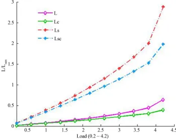
In Figure 1, with the original load of IEEE-14 standard model as a benchmark and one fifth of the original load as the step length, the load changes from 0.2 times to 4.2 times of the original load. The curve L in Figure 1 is the global L-indicator value without reactive power compensation, while Lc is global L-indicator value with reactive power compensation. Ls and Lsc in Figure 1 are the summation of all local L-indicator Lj (j = 1, 2,…, m) without and with reactive power compensation respectively. Contrasting curves L and Lc, as depicted in Figure

Figure 1. L/Lsum of IEEE-14 with load changes.

grid operation and reduce the risk of grid collapse, especially when the grid voltage stability is poorer. For ex-ample, corresponding to 3.8 of the horizontal axis, L-indicator value of L curve is close to 0.5, which means that the system is in so sensitive a state that a slight increase of load will augment the possibility of voltage instabili-ty, while L-indicator value of L curve is about 0.3 enough to avoid voltage instability. Comparing curves L and Lc to curves Ls and Lsc, what can be concluded is that the two groups of curves are the same-the shape and the trend. Therefore, L and Lc can be enlarged as Ls and Lsc, which is more convenient for observation.

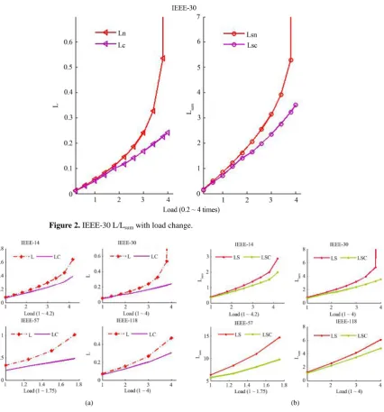
In Figure 2, the IEEE-30 standard model has been tested. The load changes from 0.2 times to 4.0 times of the original load. The effect of improving voltage stability is more apparent, and load power margin is also im-proved.

According to Figures 3(a) and (b), the conclusions obtained are similar to the above. The simulation results of the IEEE-14, IEEE-30, IEEE-57 and IEEE-118 have illustrated the universal applicability of the proposed method.

However, the difference between the above models and the actual power grids can not be ignored, which makes the voltage drop proportion of model greater than that of the actual power grids. In actual power grids, the resistance is far less than the reactance and the voltage drop caused by the active load is almost negligible. If the proposed method were applied to one model more similar to the actual power grid, the results would be more ideal.

5. Conclusion

Figure 2. IEEE-30 L/Lsum with load change.

(a) (b)

Figure 3.L(a)/Lsum(b) curves of 4 systems corresponding to each load changes.

Funding

The National Natural Science Fund Project (51107107).

Acknowledgements

We thank the support received from the National Natural Science Foundation of China (51107107) and the Chi-nese National Key Basic Research and Development Program (973) (2013CB228203).

References

[1] IEEE Committee Report (1990) Voltage Stability of Power Systems. Concepts, Analytical Tools, and Industry Expe- rience, IEEE Publication, New York.

[3] Zhou, S.X., Zhu, L.Z., Guo X.J., et al. (2004) Power System Voltage Stability Research and Control. China Electric Power Press, Beijing.

[4] Li, X.Y. and Wang, X.Y. (2003) Fast Voltage Stability Analysis Method Based on Static Equivalence and Singular Value Resolution. Proceedings of the CSEE, 23, 1-4.

[5] Jia, H.J., Yu, Y.X. and Wang, C.S. (1999) An Application of Local Indicator to Online Monitoring and Control of Power System Voltage Stability. Power System Technology, 23, 45-49.

[6] Yu, Y.X. (1999) Review on Voltage Stability Studies. Automation of Electric Power System, 23, 1-8.

[7] Zhang, J.H., Meng, X.P., Liu, H.D., et al. (2011) Analysis and Research of the Power System Voltage Stability. Power Quality Management.

[8] Liu, Y.Q., Chen, C.Y., Liang, L., et al. (2003) Review of Dynamical Analysis Art of Voltage Stability in Power Sys- tems. Proceedings of Csu-Epsa, 15, 105-108.

[9] Duan, X.Z., He, Y.Z. and Chen, D.S. (1994) Some Practical Criteria and Security Indices for Voltages Stability in Electric Power System. Automation of Electric Power System, 18, 36-41.

[10] Kessel, P. and Glavitsch, H. (Swiss Federal Institute of Technology Zurich, Switzerland) (1986) Estimating the Vol- tage Stability of a Power System. IEEE Transactions on Power Delivery.

[11] Jia, H.J., Sun, X.Y. and Zhang, P. (2006) Optimal Power Flow with Voltage Stability Constraint Based on L Index. Proceedings of Csu-Epsa.

[12] Jiang, T., Li, G.Q., Jia, H.J., et al. (2012) An Application of Simplified L-Index and Its Sensitivity for On-line Moni- toring and Control of Voltage Stability in the Large Scale Power Systems. Automation of Electric Power System, 36, 1-7.