A Hybrid Differential Evolution and Back Propagation Algorithm for Feedforward Neural Network Training

A Hybrid Differential Evolution and Back-Propagation

Algorithm for Feedforward Neural Network Training

Partha Pratim Sarangi

Seemanta Engineering College Mayurbhanj, Odisha, INDIA

Abhimanyu Sahu

Seemanta Engineering College Mayurbhanj, Odisha, INDIA

Madhumita Panda

Seemanta Engineering College Mayurbhanj, Odisha, INDIA

ABSTRACT

In this study a hybrid differential evolution-back-propagation al-gorithm to optimize the weights of feedforward neural network is proposed.The hybrid algorithm can achieve faster convergence speed with higher accuracy. The proposed hybrid algorithm com-bining differential evolution (DE) and back-propagation (BP) algo-rithm is referred to as DE-BP algoalgo-rithm to train the weights of the feed-forward neural (FNN) network by exploiting global searching feature of the DE evolutionary algorithm and strong local search-ing ability of the BP algorithm. The DE has faster exploration property during initial stage of global search for the expense of convergence speed. On the contrary, the problem of random ini-tialization of weights may lead to getting stuck at local minima of the gradient based BP algorithm. In the proposed hybrid algo-rithm, initially we use global searching ability of the DE to move towards global optimal solution in the search space for few gen-erations by selecting good starting weights and then precise local gradient searching of the BP in that region to converge to the op-timal solution with increased speed of convergence. The perfor-mance of proposed DE-BP is investigated on a couple of public domain datasets, the experimental results are compared with the BP algorithm, the DE evolutionary training algorithm and a hybrid real-coded GA with back-propagation (GA-BP) algorithm . The results show that the proposed hybrid DE-BP algorithm produce promising results in comparison with other training algorithms.

General Terms:

Pattern Recognition , Evolutionary Algorithms

Keywords:

Differential Evolution, Feedforward Neural Network, Back-propagation algorithm, Real-Coded Genetic algorithms

1. INTRODUCTION

In the past few years, pattern classification using feed-forward neu-ral networks (FNN), in specific, multilayer perceptron (MLP) is considered as promising neural network model [2] due to its ca-pability to classify the real world complex problem without prior knowledge on the problem domain. In classification, first the net-work is trained on a set of paired data from the dataset to evolve a set of free network parameters that is, selection of optimal weights

of the network weights and second, then the network is ready to test a new set of data [5].Training the weights of the multilayer percep-tron can be considered as an optimization problem in which the net-work weights are optimized. Now a days, several algorithms have been used to train the neural networks, out of these some are gra-dient based and others are evolutionary algorithms. Among them the most popular and widely used training algorithm is the back-propagation training algorithm [10, 11] , which is a gradient based approach. However, there exist some inherent problems in the propagation algorithm. First, the convergence speed of the back-propagation is slow for training a large size network. Second, for complex non-linearly separable problems or complex function ap-proximation the back-propagation algorithm easily gets stuck in lo-cal minima. Third, the training performance is very sensitive to the learning rate and momentum parameters of the algorithm. Fourth, the proper decision boundary depends on the sequence of the input data of the training set. However Curry and Morgan [6] pointed out that BP and gradient techniques may not always produce the best and fastest way to train neural networks.

parity-p problem. Some of the previous works using particle swarm optimization in [18, 19, 20, 21]for training feed-forward neural net-works.

This global search ability of EAs improves the performance of feedforward neural networks, at the expense of very high compu-tation complexity. This compucompu-tational burden includes evolution of each solution i.e. the parameters of the FNN, which requires learn-ing entire trainlearn-ing set. One of the possible methods for eliminatlearn-ing this shortcoming is to develop a hybrid algorithm which incorpo-rates the gradient descent learning followed by evolution search.

This paper is motivated by the work of Ilonen et al. presented in [1], in that authors used differential evolution (DE) proposed in [22]to train the weights of FNN. They concluded that the DE algo-rithm can converge to a global minimum for complex error surface, at the cost of very high computational complexity. In order to speed up the convergence rate and capability of avoiding local optima of DE, we proposed a simple non-Lamarckian hybrid approach by utilizing both evolutionary and gradient information. This hybrid training of FNN using the differential evolution to do global search in the beginning of training, and then the back-propagation algo-rithm to perform a local search around the global solution in the weight space of the problem to enhance the convergence speed of the training. Moreover, the experiment result shows that DE-BP training algorithm maintain better classification rate all the time without getting stuck at local minimum. Hence in this work, hy-brid DE-BP is compared with the conventional back-propagation algorithm and differential evolution based FNN training algorithm in convergence speed and generalization performance using real world bench mark datasets.

The rest of the paper is organized as follows: Section 2 deals with an overview of FNN, BP, GA, and DE algorithms respectively with a special emphasis on their strengths and weaknesses; Section 3 focuses on the detail of proposed algorithm; Section 4 describes simulation of four algorithms on 7 real world datasets with their result analysis; Section 5 provides conclusions about our work and suggestions for future work.

2. BACKGROUND STUDY

We use four algorithms for our study to train the weights of the feedforward neural network with two layered structures:the back-propagation algorithm, the differential algorithm, the hybrid ge-netic algorithms and Backpropagation, and the hybrid differential evolution and backpropagation. We briefly describe them in the fol-lowing paragraphs.

2.1 Artificial Neural Networks

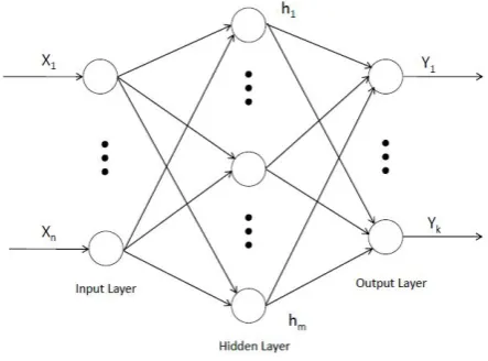
An artificial neural network (ANN) is a well-known computational model which maps input patterns from measurement space into pre-defined classes in the decision space. The feedforward neural net-works (FNN) are widely used model for pattern classification and approximate continuous functions.The most popular FNN model is multilayer perceptron (MLP) [14] comprises a set of sensory nodes that constitute the input layer, one or more hidden layer of process-ing nodes, and an output layer of processprocess-ing nodes. Fig.(1)shows three layers MLP in which neurons are structured into ordered lay-ers, and weighted connections are allowed only between adjacent layers units or neurons. The number of nodes in input layer repre-sents the coordinates of the input vector and the number of nodes in the output layer corresponds to the number of output classes. However the nodes in the hidden layer have decided optimally by trial and error basis in the experiments, these numbers of nodes

Fig. 1. Schematic representation of multilayer perceptron

vary from problem to problem. The network weights comprise both connection weights and bias term for each unit. The process of up-dating network weights is called training or learning of the neural network. For classification application supervised learning process is used, with a set of input patterns and desired outputs are used for training. The input and output of the network are both real vectors in our case.

In the supervised training change of network weights depends upon the instantaneous error between actual and expected outputs of the network. Defining the error function by the network actual output with M neurons, that is:

e=

M

X

k=1

(dk−yk)2 (1)

wheredk and yk are respectively thekth component of the

ex-pected and actual output vector. This error term can be just for one single pattern or for a set of patterns depends on on-line or batch learning. In the experiment, we use batch learning there mean square error is obtained by summing individual errors over all train-ing patterns N.

EM SE=

1

N.M

N

X

i=1

ei=

1 N.M N X i=1 M X j=1

(dij−yij)2 (2)

2.2 A brief introduction of BP

The BP algorithm is simply a gradient descent method [12, 13] de-signed to minimize the total error of the output computed by equa-tion(2) of the network in Fig.(1) using all training patterns. The total inputxh

j received by neuron j, in layer h, is defined as

xh j =

X

yh−1

i w h−1

j,i +b h−1

j (3)

Whereyh−1

i is the state of thei

th_{neuron in the preceding h-1th}

layer,wh−1

j,i is the weight of the connection from thei

th_neuron

in the layer h to thejth _{neuron in the layer h-1 andb}h−1

j is the

threshold of thejth_{neuron in layer h-1. Threshold may be added}

by giving the unit j in layer h an extra input line with a fixed activity level of 1 and a weight ofbh

The output of ajth_neuron,x

j in any layer other than the input

layer(h >0), is a parameter to a non-linear activation function of its total input and we use hyperbolic tangent activation function, defined as,

yh j =

1−e−xhj 1−e−xhj

(4)

All neurons within a layer, other than an input layer, have their states set by (1) and (2) in parallel, while different layers have their states set sequentially one after another layers forward manner until the states of the neurons in the output layer H are determined. The learning procedure determines the internal free parameters of the hidden units based on its knowledge of its inputs and the desired outputs. Hence learning consists of searching a very large parame-ter set and therefore is usually rather slow.

The least mean square (LMS) error in output vectors, for a given network is defined as,

E(w) = 1 2

X (yH

j,c(w)−dj,c)2 (5)

whereyH

j,c(w)is the state obtained for output node j in output layer

H anddj,cis its desired state specified in the supervised learning.

One method of minimization of E(w) is to apply the method of gradient descent by starting with any set of weights and repeatedly updating each weight by an amount

∆wh

ji(n+1) =η∆w h

ji(n−1)+α∆w h

ji(n−1)+hdec.w h ji(n−1)

(6) where the positive constant 0 < η < 1 controls the descent, 0 < α < 1is the damping coefficient or momentum controls acceleration, hdec is the percentage decay coefficient and n is the number of epoch currently in progress. Using a decay factor 0.01> hdec >0enables only those weights doing useful works in reducing the error to survive and hence improve the generaliza-tion capabilities of the network.

2.3 A brief introduction of GA

A genetic algorithms (GA), one of the evolutionary algorithms is a heuristic stochastic global search optimization technique that mim-ics the process of natural evolution. Like other evolutionary algo-rithms, GA is a population-based iterative search algorithm which searches from one population to another, focusing on the area of the best solution so far, while continuously searching the solution space generation wise. To achieve best solution, the GA applies stochas-tic operators such as selection, crossover and mutation. The major steps of GA include: encoding, initialization of the population, fit-ness evaluation, selection, crossover and mutation. In this work we use real valued chromosome instead of binary representation of the weights.

2.3.1 Pseudo-code of Genetic Algorithms

(1) i=0

(2) Initialize population

(3) fitness evaluation for initial population (4) while termination criteria not satisfied6=true

{

Selection Crossover Mutation

Fitness evaluation for new population

i=i+ 1;

}

end while

2.4 A brief introduction of DE

Differential evolution (DE), proposed by Storn and Price in[23], is an efficient and simple evolutionary algorithm for real parameter optimization problems. In the last few years, the DE algorithm has been successfully applied to many science and engineering appli-cations. Similar to other EAs, DE is a population based stochastic optimization method. Like other evolutionary algorithms, DE com-mences with a population of constant size of NP individual candi-date solutions, where NP is the population size. Each member is a D-dimensional real-parameters vector representing a point in the solution space S. The new candidate solutions of same population size are obtained generation by generation in the solution space. The subsequent generations are denoted by G = 0,1, Gmax. However the vectors are changed over generation wise by a spe-cial kind of differential operator instead of classical crossover and mutation operators of GA.

The number of connection weights in the network is the param-eters of a candidate solution. For L number of layers, number of parameters is.

P =

L−1 X

i=1

pi+1(pi+1) (7)

Each parameter is represented a real value in a range of (-1, 1).

2.4.1 Pseudo-code of DE Algorithm

(1) Initialize the generation G = 0 and a population PG of NP individuals randomly in the uniformly distributed range[Xmax, Xmin]

(2) WhileG < Gmax

{ fori= 1to NP do

{ Randomly generate three integer numbers r1, r2, andr3from[1, N P],wherer16=r26=r36=i

{ forj= 1to D do

mutation:Generateith_{donor vectorV} i,

vi,j=xr1,j+F∗(xr2,j−xr3,j)

. Rearrangement:keep each parameters of donor vector in the range[Xmin, Xmax].

crosover:Generateith_{trial vectorU} i

If rand (0,1) < CR, then ui,j = vi,j Else

ui,j=xi,j

}end

Selection and replacement:

If individualuifitness is better than individualxi,

then Replace individualxibyuiindividual

} }end end

Fig. 2. Framework of hybrid algorithm for classification

2.5 Hybrid Algorithms

To overcome the local minima problem of BP due to initial ran-dom weight parameters of the network a number of evolutionary algorithms has been tried by many researchers, which improve the performance of the classification at the cost of more execution time. In this work we hybridized two algorithms, combining global search evolutionary algorithm and local search gradient algorithm that overcomes the local minima problem with high generalization and fast convergence speed. We tried two hybrid algorithms: a GA with the BP (GA-BP) algorithm and a DE with the BP proposed (DE-BP) algorithm.

3. PROPOSED DE-BP ALGORITHM

The hybrid DE-BP is a training algorithm combining the DE algo-rithm with the BP. Similar to the GA, the DE is an evolutionary population based global optimization algorithm, which has strong ability to explore the entire search Space. This algorithm has a dis-advantage that the search around the global optimum solution is very slow. In contrary, the BP has precise and fast local searching ability to explore locally the optimum result, but it suffers to find global optimum result in complex search space.

By combining the evolutionary DE and the gradient based BP algorithm, a new algorithm referred to as hybrid DE-BP algo-rithm, illustrated in Fig.(2). The proposed hybrid algorithm has two stages: first one a global search phase, the FNN is trained using the DE algorithm for few pre-defined generations or training error is smaller than some predefined value, then training process switched to second phase for searching locally using a deterministic method such as the back-propagation algorithm. In this work, it realized DE-BP hybrid training algorithm as a successful alternative ap-proach to BP algorithm.

The DE-BP algorithm’s searching process is started from ini-tializing a group of random target vectors as population. First, all the target vectors are updated using mutation operator and produce donor vectors. In the crossover, for each donor vector and for all components check if rand (0, 1) ¡ CR then change the donor vec-tor component else that component will remain in the donor vecvec-tor and finally trial vectors are generated. Then selection offspring by fitness value of each trial vector is compared with the

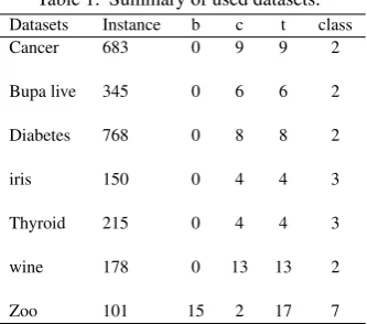
correspond-Table 1. Summary of used datasets. Datasets Instance b c t class

Cancer 683 0 9 9 2

Bupa live 345 0 6 6 2

Diabetes 768 0 8 8 2

iris 150 0 4 4 3

Thyroid 215 0 4 4 3

wine 178 0 13 13 2

Zoo 101 15 2 17 7

ing target vector, best fit vector will be selected as new offspring for next generation and then those new target vectors are used to search the global best position in the solution space. Finally the BP algorithm is used to search around the global optimum. In this way, proposed hybrid algorithm improves the convergence speed than the DE algorithm and less chance to get stuck in local minima like the BP algorithm.

The pseudo code for this hybrid DE-BP algorithm can be sum-marized as follows:

STEP 1: Initialize the DE parameters.

STEP 2: Initialize the population with real values in the domain [0,1] for each neuron’s connection weights and bias to its corresponding gene segments .

STEP 3: While new gen. is less than equal to MaxGen.DO{

STEP 4: The fitness of target vectors are determined by MSE STEP 5: Sort minimum fitness values.

STEP 6: If first fitness value is less than equal to min. error then select best solution for MLP then goto step.9

STEP 7: Generate donor vectors of the population using mutation. STEP 8: Generate trail vectors of the population using crossover STEP 9: Selection of new offspring of the population for new

generation}

STEP 10: Initialize parameters of back-propagation learning STEP 11: Initialize weights of the MLP using best solution of

RGA

STEP 12: While new epoch is less than equal to MaxEpoch or error converges to Min Error do

STEP 13: Update weights to minimize error using back-propagation with training data

STEP 14: End while

STEP 15: Evaluate performance of classification with test data STEP 16: End while

4. EXPERIMENTAL STUDY

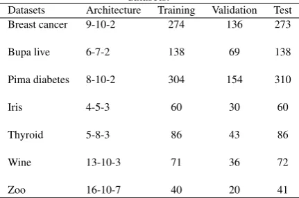
Table 2. FNN Architecture and patterns distribution of all datasets.

Datasets Architecture Training Validation Test Breast cancer 9-10-2 274 136 273

Bupa live 6-7-2 138 69 138

Pima diabetes 8-10-2 304 154 310

Iris 4-5-3 60 30 60

Thyroid 5-8-3 86 43 86

Wine 13-10-3 71 36 72

Zoo 16-10-7 40 20 41

4.1 Experimental real world datasets

We use seven datasets from different classes as summarized in table 1 to compare the performances of BP algorithm, DE based training algorithm, GA-BP algorithm and DE-BP algorithm in optimizing the weights of the FNN. These data sets are the Wisconsin breast cancer, bupa liver diagnoses, pima diabetes, fisher’s iris plant, thy-roid dysfunction, wine and zoo data sets. Table 1 lists a summary of the used datasets along with following attributes: datasets and the number of instances, the number of binary (b), continuous (c) fea-tures in the dataset, the total (t) number of feafea-tures, and number of classes. The data sets were obtained from the UCI repository [24].

In this paper, we use FNN in particular multi-layer perceptron (MLP) with three layers (input-hidden-output). The number of neu-rons in the input and output layers of the FNN depends on the fea-tures and classes of the concerned data set used in the experiment. The performance of the FNN gets affected by number of neurons in the hidden layer. We adopt trial and error process to decide the number of neurons in the hidden layer by considering the perfor-mance of the FNN. Table 2 summarizes the network architecture for each data set.

In the classification problems, the data sets are used to deter-mine the class that a certain input vector belongs to. Each pattern from the training set consists of an input vector and its desired out-put vector. These inout-put and outout-put vectors are normalized and rep-resented as real vectors. The size of the input and output vectors are depended on number of features and classes present in the data set. When an input vector is assigned to the FNN, the network re-sponse is one of the classes associated with the output neuron hav-ing greater value.

To evaluate a FNN, each data set splits into three parts: the training patterns, the validation patterns and the test patterns [16]. The first two sets are used for training algorithm and last one is used for testing. The forty percent of the data set for training, twenty percent for the validation and remaining forty percent for testing. A popular and very useful form to use validation set in neural net-work is early stopping. Indeed the validation set used for testing the performance of the network in the training phase and it is nec-essary to avoid the overtraining phenomenon. Before partition of the dataset, it is normalized in the range of [0, 1]. We run all the al-gorithm of our experiment ten times for every data set and evaluate average performance of the FNN.

The proposed algorithm DE-BP is compared with BP algorithm and DE based training algorithm, GA-BP algorithm and DE-BP proposed one were implemented and analyzed using matlab.

4.2 EXPERIMENTAL PREPARATION

The following steps summarized the preparation of the experiment and configuration parameters of all algorithms.

(1) Before partition of the data set, patterns are normalized (2) Then partition of the data set randomly into two groups: sixty

percent of training and forty percent of test patterns

(3) Again training patterns is partitioned into two groups: forty percent of training and twenty percent of validation

(4) Synaptic weights of the MLP are randomly initialized by real values in a domain [-1, 1]

(5) Configuration parameters of MLP like learning rate (η) = 0.001, momentum(α) = 0.9 and decay coefficient (hdec) = 0.0002

(6) Training stops by three ways: (1) TheGL5stopping criterion; (2) training error ¡ 0.001; (3) the maximum number of itera-tions is satisfied

(7) Each candidate solution in the population represents the neural network architecture

(8) The length of the candidate solution is the total number of con-nection weights of the network

(9) The real-coded GA and DE algorithm use real parameters to represent candidate solutions

(10) Population size is 100 for all three algorithms: DE, GA-BP and DE-BP

(11) DE algorithm use DE/best/1/bin strategy

(12) If the elements of the donor vectors are out of search space then repair operator is used

(13) In DE to increase the potential diversity of the population, a crossover operator is used, binomial crossover has used with Crossover rate: 0.7

(14) Elitism the best solution means lower fitness value is pre-served for the next generation

(15) Number of generationsin each experimentfor GA-BP and DE-BP is 100

(16) The GA-BP algorithm uses rank-based selection

(17) The GA-BP algorithm uses arithmetic crossover with crossover rate 0.7

(18) The GA-BP uses non-uniform mutation with mutation rate 0.01

(19) Each classifier repeatedly executes ten times over all datasets (20) NMSE and accuracy of the classifiers compared in table 3, 4

and 5.

4.3 EXPERIMENTAL RESULT ANALYSIS

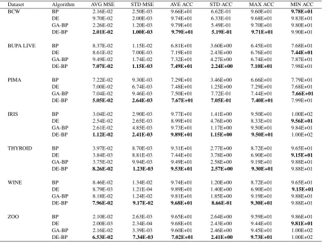
Table 3. Average,Standard deviation,min;and max of NMSE and accuracy for all training samples over ten independent runs for BP, DE, GA-BP, and DE-BP

Dataset Algorithm AVG MSE STD MSE AVE ACC STD ACC MAX ACC MIN ACC

BCW BP 2.16E-02 2.50E-03 9.66E+01 6.62E-01 9.60E+01 9.78E+01

DE 9.70E-02 2.00E-03 9.74E+01 6.33E-01 9.68E+01 9.83E+01

GA-BP 2.26E-02 1.20E-03 9.79E+01 5.49E-01 9.70E+01 9.80E+01 DE-BP 2.01E-02 1.00E-03 9.79E+01 5.19E-01 9.71E+01 9.90E+01

BUPA LIVE BP 8.37E-02 1.15E-02 6.81E+01 3.60E+00 6.45E+01 7.68E+01

DE 8.61E-02 7.00E-03 7.19E+01 2.43E+00 6.76E+01 7.44E+01

GA-BP 9.49E-02 1.74E-02 7.32E+01 4.27E+00 6.74E+01 7.87E+01 DE-BP 7.07E-02 1.15E-03 7.49E+01 2.24E+00 7.10E+01 7.98E+01

PIMA BP 7.22E-02 9.30E-03 7.29E+01 3.46E+00 6.66E+01 7.79E+01

DE 7.00E-02 6.74E-03 7.48E+01 1.25E+00 7.29E+01 7.68E+01

GA-BP 7.04E-02 9.46E-03 7.50E+01 7.72E-01 7.44E+01 7.66E+01

DE-BP 5.05E-02 2.64E-03 7.67E+01 7.05E-01 7.40E+01 7.99E+01

IRIS BP 3.04E-02 2.90E-03 9.77E+01 1.41E+00 9.50E+01 1.00E+02

DE 2.54E-02 2.65E-03 8.99E+01 4.76E+00 8.33E+01 9.56E+01

GA-BP 2.61E-02 4.85E-03 9.73E+01 1.17E+00 9.50E+01 9.84E+01 DE-BP 1.12E-02 2.41E-03 9.89E+01 1.15E+00 9.50E+01 1.00E+02

THYROID BP 3.97E-02 8.70E-03 9.31E+01 2.77E+00 8.72E+01 9.65E+01

DE 3.84E-03 8.81E-03 7.44E+01 3.78E+00 6.90E+01 9.15E+01

GA-BP 3.75E-02 9.94E-03 9.49E+01 2.58E+00 9.19E+01 9.88E+01 DE-BP 8.26E-02 1.23E-03 9.53E+01 2.57E+00 9.30E+01 9.88E+01

WINE BP 8.46E-02 1.34E-02 9.74E+01 1.20E+00 8.72E+01 9.65E+01

DE 8.79E-03 1.21E-04 9.89E+01 1.40E+00 6.90E+01 9.15E+01

GA-BP 8.18E-02 1.24E-02 9.81E+01 1.85E+00 9.19E+01 9.88E+01 DE-BP 7.96E-02 9.17E-02 9.68E+01 8.66E-01 9.30E+01 9.88E+01

ZOO BP 2.10E-02 2.63E-03 9.65E+01 2.64E+00 9.59E+01 9.86E+01

DE 2.00E-03 2.34E-04 9.68E+01 2.43E+00 9.44E+01 9.81E+01

GA-BP 2.16E-02 3.39E-03 9.60E+01 2.46E+00 9.45E+01 1.00E+02 DE-BP 6.53E-02 7.34E-03 7.02E+01 2.41E+00 9.73E+01 1.00E+02

results in the most dataset where DE based training fails. By tak-ing advantage of global optimization, early stopptak-ing, and weight decay proposed algorithm takes less computational time than DE based training algorithm. Similarly, the problem of local minimum of BP algorithm observed many times in running the training algo-rithm number of times over all datasets. It leads worst performance in the experiments that could be avoided by proposed algorithm. From the experiments, it has revealed that by a large population size the DE training algorithm needs small number of generations to improve its performance. Here we used 50 to 200 population size and achieved better results. In the proposed algorithm popula-tion size used 100.Then BP algorithm takes small number of epochs to optimize the connection weights of FNN with less mean square error. In DE based training, maximum generation number was cho-sen 500. It is analyzed from Table 2 that for almost all datasets the classification rate of the proposed training algorithm outperforms classical back-propagation and DE method. All most all Datasets like bupa, diabetes, iris, thyroid, wine and zoo the proposed algo-rithm obtained better results than BP and DE method. Moreover in breast cancer dataset DE based training produced best result than proposed training algorithm. Thus it is clearly observed from the ta-ble that where BP and DE based training not performed well there

proposed training algorithm obtained best results. However it has also analyzed from the experiments that DE did not perform well except breast cancer dataset and time needed for convergence al-ways more than BP and proposed algorithm. Hence, no advantage is found in this study to use DE as global optimization training al-gorithm over conventional BP. But from the results we realized that the proposed algorithm, initially DE evolved a better search space globally in few generations then BP locally searched around the global position to optimize the connection weights of the neural network.

5. CONCLUSION

a

b

c

e

f

g

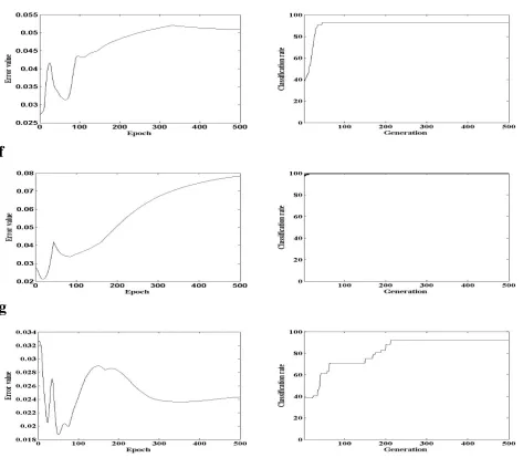
Fig. 3. The training error curves and rate of accuracy curves of De-BP based on average MSE for all training samples over ten independent run in seven datasets (a),(b),(c),(d),(e),(f)and (g) respectively.

The back-propagation algorithm not always performs better and traps in local minima. However, when problems are more complex, back-propagation most often fails because of non-differentiable er-ror functions. The experimental results of the proposed hybrid al-gorithm improve the training error convergence and classification accuracy than others. Moreover, the proposed algorithm produces higher classification accuracy in less training time than the DE gorithm and BP algorithm. The results of proposed hybrid DE al-gorithm are quite convincing in fast error convergence and stable classification accuracy than hybrid GA algorithm.

Finally, from the experiments, we can conclude that DE-BP takes less CPU time, with maintaining higher training accuracy

than other three algorithms. From the experiments, it can also see that DE-BP algorithm has smooth MSE and accuracy rate than other algorithms. In future research works, we shall focus on how to extend this work to solve more real world problems.

6. REFERENCES

[1] J. Ilonen, J. K. Kamarainen, and J. Lampinen: Differen-tial evolution training algorithm for feed-forward neural net-works, Neural Processing Letters, 17:93-105, 2003.

Algorithm”,International Journal of Computer Applications 51(18):30-36, 2012

[3] H. Hasanrkc, HasanBal, ”Comparing performances of back-propagation and genetic algorithms in the data classification”, Expert Systems with Applications, Volume 38, Issue 4,Pages 3703-3709, 2011.

[4] Zhang, G., ”Neural networks for classification: a survey”, IEEE Transactions on Systems,Man, and Cybernetics, Part C 30(4): 451-462, 2000.

[5] S. B. Kotsiantis, ”Supervised Machine Learning: A Review of Classification Techniques”, Informatica31 249-268, 2007 [6] Curry B, Morgan P. Neural networks: a need for caution.

Omega, International Journal of Management Sciences, 1997 [7] D. J. Montana and L. Davis, Training Feedforward Neu-ral Networks using Genetic Algorithms, Proceedings of the Third International Conference on Genetic Algorithms, Mor-gan Kaufmann, San Mateo, CA, 379-384,1989

[8] Sexton, R., Dorsey, R., and Johanson, J., ”Optimization of Neural Networks: A Comparative Analysis of the Genetic Al-gorithm and Simulated Annealing”, European Journal of Op-erational Research, volume 114, issue 3,page 589-601,1999. [9] Sexton, R., Dorsey, R., and Johanson, J., ”Toward a Global

Optimization for Neural Networks:, A Comparison of the Ge-netic Algorithm and Backpropagation”, forthcoming in Deci-sion Support Systems.

[10] Gupta, J. N. D., and Sexton, R. S. Comparing back-propagation with a genetic algorithm for neural network train-ing. Omega, 27, 679-684.

[11] X. Yao, Evolving artificial neural networks, Proc. IEEE 87 (9), 1423-1447, 1999.

[12] Werbos P. The roots of the backpropagation: from ordered derivatives to neural networks and political forecasting. New York: John Wiley and Sons, Inc, 1993

[13] D.E. Rumelhart, G.E. Hinton, R.J. Williams, Learning repre-sentations by back-propagating errors, Nature 323 533-536, 1986

[14] Simon Haykin, ”Neural Networks: A comprehensive founda-tion,” Pearson Education Asia, Seventh Indian Reprint, 2004. [15] D. Whitley, ”Applyong Genetic Algorithms to Neural Net-work Problems,” International Neural Network Society pp.230, 1988.

[16] Prechelt, L.: Proben1, ”A Set of Neural Network Benchmark Problems and Benchmarking Rules”. Technical Report 21, FakultatfurInformatik University at Karlsruhe, 76128 Karl-sruhe, Germany, 1994.

[17] Schaffer J. D., D. Whitley, and L. J. Eshelman, ”Combina-tions of Genetic Algorithms and Neural Networks: A Survey of the State of the Art, ” Proceedings of the IEEE Workshop on Combinations of Genetic Algorithms and Neural Network. [18] C. Zhang, H. Shao. and Y. Li. ”Panick swarm optimization for evolving artificial neural network”, Procccdings of the IEEE lntcrnational Conference 011 System, Man, and Cybcmctics. vol. 4, pp.24x7-2490, 2000.

[19] Zhang, J. R., Zhang, J., Lok, T. M., and Lyu, M. R. (2007). A hybrid particle swarm optimization-back-propagation algo-rithm for feedforward neural network training. Applied Math-ematics and Computation 185, 1026 - 1037.

[20] Zhang, C., and Shao, H., An ANN’s evolved by a new evolu-tionary system and its application. In Proc. of the 39th IEEE conf. on decision and control. vol. 4, pp. 3562 - 3563, 2000.

[21] M. Sellcs and B. Rylander, ”Neural network learning using particle swarm optimization”, Advances in Information Sci-ence and SoftComputing. pp. 224-226, 2002

[22] R. Storn, and K. Price, ”Differential Evolution-A Simple and Efficient Heuristic for Global Optimization over Continuous Spaces, ” Journal of Global Optimization, Vol. 11, pp. 341-359, 1997.

[23] Adam Slowik, and Michal Bialko, ”Training of Artificial Neural Networks Using Differential Evolution Algorithm”, Krakow, Poland, May 25-27, 2008