Measured Data of Hourly Global Solar Irradiation Using Two Curve Fitting Methods

(1)

Page 202

Measured Data of Hourly Global Solar Irradiation Using Two

Curve-Fitting Methods

Aditi Pareek

1

_{, Dr.Lata Gidwani}

2

1

_{Department of Renewable energy and Electrical Engineering, University college of Engineering, Rajasthan}

Technical University Kota, Rajasthan, INDIA.

---***---Abstract - Solar energy has an important role to

achieve the goal of replacing fossil fuels and significant potential to reduce green house gas emissions. Accurate information on solar radiation is very essential for engineers, architects and agriculturist to design the energy systems based on the solar source. The radiation data is highly useful for the designing of solar energy related electricity generation systems. The data was filtered by using polynomial fitting method. This paper studies the use of polynomial fitting to the global solar radiation that was measured by using Pyranometer model no. CMP11 at Kolayat, located in Rajasthan, India. Measured hourly global solar radiation data of Kolayat in May 2015 were analyzed in this work. The two curve –fitting methods that were found to be suitable to be applied to the filtered solar radiation data is the polynomial fit and the sinusoidal fit. Author have been takensolar radiation data every five minute during 6:00-20:00 . The polynomial data fitting method was used for data smoothing and was tested by using different degrees of polynomial curve fittings. The error measurement was calculated by using the root mean square error (RMSE) and by determining the R2_{value. The polynomial fittings were}

carried out by using MATLAB.

Key Words:

Curve-fitting; polynomial fit and

sinusoidal fit; Global solar radiation data; Matlab

1. INTRODUCTION

The demand for energy is increasing exponentially as the human population increases dynamically [1-2].The solar radiation is an instantaneous power density measured in units of kW/m2_{. In providing alternative energy sources} and in electricity generation solar radiation prediction and forecasting plays a vital role [3]. In Karim et al. [4] the best polynomial fitting degree for solar radiation data is calculated using RMSE (root mean square error) and r2 value. The curve fitting methodology requires the interpolation or approximation of the given data sets which are subjected to certain constraints such as continuity, error measurement, etc. Karim and Piah [5]

and Karim et al. [6] have discussed the applications of curve fitting methods (interpolating and approximating method) in font designing and shape preserving interpolation which can be considered as important in certain applications. The rest of this paper is structured as follows. In section II solar radiation data collection and solar radiation Data using Polynomial fitting is discussed. Section III presents the Data fitting model frame work. Results are discussed and summarized In Section IV. Finally, In Section V conclusions are drawn.

2. SOLAR RADIATION DATA COLLECTION

The emitted solar radiation is the electromagnetic

Radiation that is emitted by the sun in the wavelength Region of 280 nm to 4000 nm [1]. The instantaneous

global solar radiation value at STP is estimated to be 1000 W/m2_{, while the value of power density outside the earth’s} atmosphere is 1353W/m2_{[7]. At Kolayat, the data is} measured by using Pyranometer model no. CMP11 as shown in Figure1. Data is captured by using computerized data acquisition system.10MW solar power plant as shown in Figure 2.

(2)

Page 203

Fig-1(b): Pyranometer CMP11

[image:2.595.43.287.83.492.2]

Fig-2: 10 MW Solar Power Plant, Kolayat, Rajasthan

2.1 Polynomial data fitting

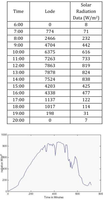
Polynomial data fitting is used for filtering and smoothening of global solar radiation data received in the stations. It was tested by various degrees of solar radiation data. The literature for doing curve fitting is well established and can be found in [8–12]. The solar radiation data is obtained shown in Table 1 and it is represented graphically in Fig3. There are various degrees of polynomial curve fitting such as linear polynomial, quadratic polynomial, cubic polynomial, 4th_degree polynomial, 5th_{degree polynomial, 6}th_{degree, 7}th _degree, 8th_{degree, 9}th_{degree polynomial and so on. These} polynomials are applied on the received solar radiation data for a perfect fitting. . Table 3 shows all the polynomial fitting results. Rmse which gives an error value and r2 (coefficient of distribution) gives the goodness of fitting of data.

Table -1: Daily Average of Measured Global Solar Radiation Data (KOLAYAT 09 -MAY 2015)

Time Lode

Solar Radiation Data (W/m2₎

6:00 0 8

7:00 774 71

8:00 2466 232

9:00 4704 442

10:00 6375 616

11:00 7263 733

12:00 7863 819

13:00 7878 824

14:00 7524 838

15:00 4203 425

16:00 4338 477

17:00 1137 122

18:00 1017 114

19:00 198 31

20:00 0 7

Fig- 3: Graphical Representation (09-MAY 2015)

[image:2.595.325.540.129.546.2]

(3)

[image:3.595.28.293.138.465.2]

Page 204

Table-2: Measured Peak Solar Radiation Data Every Five

Minute (Kolayat 09-May 2015)

Time Lode Radiation

Data (W/m2₎

Time Lode Radiation

Data (W/m2₎

12:05 7965 833 13:05 8034 867

12:10 7782 815 13:10 8013 862

12:15 7887 829 13:15 8010 874

12:20 7860 825 13:20 8001 872

12:25 7743 798 13:25 7893 862

12:30 7983 841 13:30 7860 864

12:35 7836 824 13:35 7887 865

12:40 7752 817 13:40 7650 856

12:45 7266 763 13:45 7684 848

12:50 6177 630 13:50 7719 842

12:55 7242 743 13:55 7626 841

From Wu and Chan [3], we believe the best model for the fitting of solar radiation data is quadratic polynomial shown in Fig.5(b) Since it gives better indication to the solar radiation data compare with other polynomial fitting model. Polynomial of nth _degree

y= a0 + a1x + a2x2 +……+ an xn (1)

This can be achieved by defining the error of fitting model:

ei y f xi i yi a a xi a xi a xn i n

= - ( )= -

n

0+ 1 + 2 2+ +....

s

₍₂₎

Taking sum square of the error in (2) gives us

S i e y a a x a x a x

N

i _i

N

i i i i n in

= = - + + + +

=0 =

2

0 0 2

2 _... 2

n

s

(3) To obtain least square fitting, the sum of error in (3) must be minimized. Hence,

 

s

a_i=0,i=0,1,.... .n ₍₄₎

The values of a0, a1, …….., an which gives the best least square polynomial equation for the given data.

ᵡ_{= Chi Square} yi = actual value

xi = calculated Y fit value σi = weight

y = mean of actual values

x _{= mean of calculated Y fit values}

R = i

 

( )( )

( ) ( )

x x y y

i i

i i i i

-

-- 2 - 2

(5) R y y i i i =

-1 2 ₂

( ) (6)   2 2

=

F

-H

G

I

_K

J



i i i i y x (7)

3. DATA FITTING MODEL FRAMEWORK

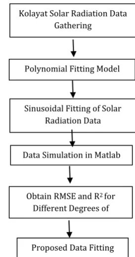
This section will gives framework for solar radiation data fitting. Figure 4 shows the framework.

Fig-4: Data Fitting Frame work

Figure 4 shows the basic block diagram which describes the flow of polynomial data fitting and sinusoidal fitting methods.

4. RESULTS AND DISCUSSION

Author apply polynomial fitting (regression) starting with degree 1 (linear) until degree 9th_{. All the polynomial}

Kolayat Solar Radiation Data Gathering

Polynomial Fitting Model

Sinusoidal Fitting of Solar Radiation Data

Data Simulation in Matlab

Proposed Data Fitting Model

ObtainRMSE andR2 _for

[image:3.595.380.517.365.624.2]

(4)

Page 205

coefficients are calculated based on 95% confidence

interval. Table 3 summarized all the polynomial fitting results. Figs. 5 (a) until 5 (i) shows the polynomial fitting for solar radiation data.

Table-3:

Polynomial fitting

Polynomial Fitting Statistics

RMSE R2

n=1

y=0.26*x+3.8e+02

297.7 0.00916

7 n=2

y = - 0.0069*x^{2}

+ 5.2*x - 2.1e+02

65.28 0.9568

n=3

Y=-4.3e-06*x^{3}-

0.0023x^{2}+3.9x-1.3e+02

61.35 0.9657

n=4

y = 4.3e-08*x^{4} -

6.6e-05*x^{3}

+

0.026x^{2} - 0.61x +

26

60.28 0.9759

n=5

y = 5.5e-11*x^{5} -

5.7e-08x^{4}-2.1e-06x^{3}+0.009*x^{2}

+ 1.1*x -13

48.84 0.9767

n=6

y = 3.9e-13*x^{6} -

7.8e-10*x^{5}+6.3e-

07x^{4}-0.00026x^{3}+

21.68 0.9962

0.056x^{2} - 2.2x +

40 n=7

y = 5.5e-16*x^{7} -

1e-12*x^{6}

+

6e-

10*x^{5}-6.3e-

08x^{4}-8.4e-05x^{3}+ 0.033*x^{2}

- 0.99*x +26

20.61 0.9994

n=8

y = - 1.9e-18*x^{8}

+6.2e-15*x^{7} -

7.6e-12*x^{6}

+

4.7e-

09x^{5}-1.5e-06x^{4}+0.00018*x^{

3}

+0.0071*x^{2}+

0.028*x + 17

20.09 0.9994

n=9

Y= 6e-23*x^{9} -

2.8e-19x^{8} + 4e-16x^{7}

- 6.4e-15*x^{6} -

5.2e-10x^{5} + 5e-07x^{4}

-0.00019*x^{3}

+

0.031x^{2} - 1.9x +

29

(5)

Page 206

(a)

(b)

(c )

(d)

(e)

(6)

Page 207

(g)

(h)

(i)

Fig-5: Various polynomial fitting (a) n=1 (b) n=2 (c) n=3 (d) n=4 (e) n=5 (f) n=6 (g) n = 7 (h) n = 8 (i) n = 9

From Figs. 5(a) until 5 (i), it can clearly be seen that once the degree of the polynomial is increasing, the fitting graphs will starting to wiggle. Among the entire fitting model, quadratic, cubic and quartic polynomials seem to give better results as compare with the other fitting model.For polynomial fitting with degree are quadratic, cubic and quartic, the value of RMSE and R2 _{can be} obtained in Table 3. From the table, Polynomial fitting with 9th _{degree gives better R}2_{(0.9996) and RMSE is} 10.09.

Fig.6: Sinusoidal fitting

There is trade-off between less RMSE and higher R2 value. From figure6 Sinusoidal fitting gives better R2 (0.9328) and RMSE is 74.98.

5. CONCLUSIONS

(7)

Page 208

ACKNOWLEDGEMENT

The author would like to thank NVR Infrastructure and Services Pvt. Ltd. for its data support.

REFERENCES

[1]

Karim, S.A.A., Singh, B.S.M, Karim, B.A., Hasan, M.K., Sulaiman, J., Josefina, B. Janier., and Ismail, M.T. (2012). Denoising Solar Radiation Data Using Meyer Wavelets. AIP

Conf.Proc.1482:685-690.

http://dx.doi.org/10.1063/1.4757559.

[2] Karim, S.A.A., Singh, B.S.M., Razali, R. and Yahya, N. Data Compression Technique for Modeling of Global Solar Radiation. In Proceeding of 2011 IEEE International

Conference on Control System, Computing and

Engineering (ICCSCE) 25-27 November 2011, Holiday Inn, Penang, pp. 448-35,(2011a).

[3] Wu, J. and Chan, C.K. Prediction of hourly solar radiation using a novel hybrid model of ARMA and TDNN. Solar Energy 85:808-817, 2011.

[4] Samsul Ariffin Abdul Karim and Balbir Singh

Mahinder Singh,’’ Global Solar Radiation

Modeling Using Polynomial Fitting’’ Applied

Mathematical Sciences, Vol. 8, 2014, no. 8, 367 – 378.2012.

[5] Karim, S.A.A and Piah, A.R.M (2009). Rational Generalized Ball Functions for Convex Interpolating Curves. JQMA 5(1): 65-74.

[6] Karim, S.A.A., Karim, B.A., Hasan, M.K. and Sulaiman, J. (2010d).Font Designing Using Generalized Ball Basis. In Proceedings of EnCon2010, 3rd Engineering Conference on Advancement in Mechanical and Manufacturing for Sustainable Environment April 14-16, 2010, Kuching, Sarawak, Malaysia, ISBN 978-967-5418-10-5.

[7] Thekaekara, M.P. (1973). Solar Energy Outside the Earth’s Atmosphere. Solar Energy 14. p. 109.

[8] R.E. Childs, Donald G.S. Chuah, S.L. Lee, K.C. Tan. Analysis of solar radiation data using cubic splines. Solar Energy,Volume32 ,Issue 5, 1984, Pages 643-653.

[9] Donald G. S. Chuah, S. L. Lee. Solar radiation in peninsular Malaysia—Statistical presentations. Energy

Conversion and Management, Volume 22, Issue 1, 1982,

Pages 71-8.

[10] Genc, A., Kinaci, I., Oturanc, G., Kurnaz, A., Bilir, S. and Ozbalta, N. Statistical Analysis of Solar Radiation Data Using Cubic Spline Functions. Energy Sources, Part A:

Recovery, Utilization, and Environmental Effects. 24:12 1131-1138. (2002).

[11] De Boor, C. 2001. A Practical Guide to Splines. Springer-Verlag New York.

[12]Dr.P.M.BeulahDevamalar,Dr.V.ThulasiBai,D.Jahnavi, V.Vidhyawathy, Gap Filling of Solar Radiation Data using Polynomial Fitting and Wavelet Transform Comparison, International Journal for Scientific Research & Development, Vol. 2, Issue 12, 2015 | ISSN (online): 2321-0613 pp.no.268-270.

BIOGRAPHIES

Aditi Pareek received the B. tech .degree in Electronics Instrumentation and control Engineering from the Global Institute of technology (GIT), jaipur India in 2011. She is currently working toward the M. Tech. degree in Renewable Energy Technology at Department of Renewable Energy, Rajasthan Technical University, Kota, India. Her current interests include Solar Energy, Artifical Neural Networks Technique, optimal control.

Dr. Lata Gidwani received her B.Tech in Electrical Engineering from CTAE, Udaipur, India in 2000 and M. Tech. in Power Systems from MNIT, Jaipur, India in 2002. She has done Ph.D. from MNIT, Jaipur, India in 2012. She is currently working as Associate Professor in Electrical Engineering

Department, Rajasthan Technical

University, Kota, India. She has

Measured Data of Hourly Global Solar Irradiation Using Two Curve Fitting Methods

Page 202