Optimization of Convolutional Neural Network Target Recognition Algorithm

14th International Conference on Wireless Communications, Networking and Mobile Computing (WiCOM 2018) ISBN: 978-1-60595-578-0

Optimization of Convolutional Neural Network Target Recognition Algorithm

ABSTRACT

This paper proposes an optimized convolutional neural network target recognition algorithm for the problem of low recognition rate of synthetic aperture radar (SAR) target training, under the condition of insufficient tag data, translation, rotation and complexity. In order to overcome the shortage of tag data, the convolutional neural network is initialized with a feature set, obtained by principal component analysis (PCA) unsupervised training. In order to improve the training speed while avoiding overfitting, Rectified Linear Unit (ReLU) function is used as the activation function. In order to enhance robustness and reduce the effect of down sampling on feature representation, this work uses a maximum probability sampling method and normalizes the local contrast of feature after convolution layers. The experimental result shows that, compared with traditional convolutional neural network, this approach achieves a higher recognition rate for SAR target and better robustness to various image deformation and complex background.

Keywords：Convolutional neural networks; Deep learning; principal component analysis

INTRODUCTION

Accurate and robust target recognition in images is the core of pattern recognition and artificial intelligence. In the military field, with the improvement of the synthetic aperture radar (SAR) imaging technology and the rapid growth of SAR datasets, acquiring and identifying various military targets from large amounts of data and complex scenes have become a research hotspot. In recent years, deep neural network (DNN) has become a new hot area in machine learning. The image recognition algorithm based on convolutional neural network (CNN) has been paid great attention by academic and industry because of its strong robustness and outstanding recognition rate.

Osendorfer et al. [2] proposed a natural image recognition algorithm based on large and deep CNN, which obtained a high recognition rate on the ImageNet data set. Roth et al. [3] suggested a multi-core CNN and a graphics processing unit (GPU) parallel algorithm, which had a good recognition effect on the 3-dimentional

NORB dataset. Even though all the above algorithms have achieved high recognition rates, they are all supervised learning approaches, which means that the adjustment of network weights requires large quantities of tag data in practice. The models cannot be fully trained with small data size, so they only apply to large datasets, which has plenty of tag data. The current mainstream solution to this problem is to initialize CNN with the filter sets, obtained by using feature extraction algorithm for unsupervised pre-training. Ozekiet al. [4] used

sparse coding to extract the basis function of the input data, and then used it as the initial filter of the network. Burges et al. [5] used independent component analysis (ICA) pre-training to initialize the weight parameters of CNN. Both initialization methods have achieved certain improvement in the recognition rate, but their effects on data feature extraction are relatively modest. Therefore, it is necessary to explore a more efficient and robust algorithm for unsupervised learning.

In addition to weight initialization, the pooling layer is also an important factor that affects the recognition rate and robustness of the CNN. The pooling layer mainly aims to obscure and generalize features, to obtain the invariability of translation and scale. The state of the neuron in this layer is determined by local receptive field of the previous layer and the sampling rules, which usually take the minimum, maximum, medium or mean of the neuron response value in the receptive field. However, this process is irreversible. Some data features will be lost during the back propagation process, which directly limits the recognition rate and robustness of the network. Lécun et al. [6] used maximum sampling. And after passed through two convolution layers and two pooling layers, the output value has a certain loss relative to the original input data. This has a direct effect on the recognition accuracy. Nebauer et al. [7] optimized the original downsampling method, and proposed the maximum probability sampling method to preserve the feature information to the greatest extent, while guaranteeing the invariance.

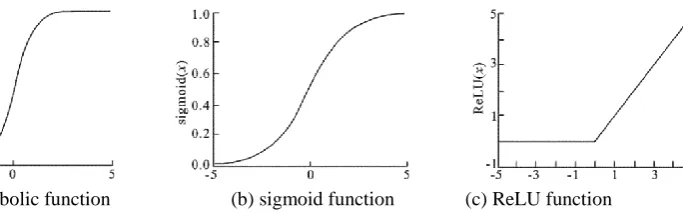
In view of the above problems, this paper proposes a CNN target recognition algorithm based on principal component analysis (PCA). First, the PCA unsupervised pre-training is used to initialize the network. By minimizing the reconstruction error, the hidden layer representation of the images can be obtained. And then the filter sets, which have the statistical characteristics of the training data, can be learned. Secondly, in order to improve the training speed and sparse feature while avoiding overfitting, the Rectified Linear Unit (ReLU) function is used as the nonlinear function. In order to enhance robustness and reduce the loss of feature information caused by down sampling, this work uses the maximum probability sampling method and normalizes the local contrast of feature after convolution layers.

APPROACH

A. Principle Component Analysis (PCA) Unsupervised Training

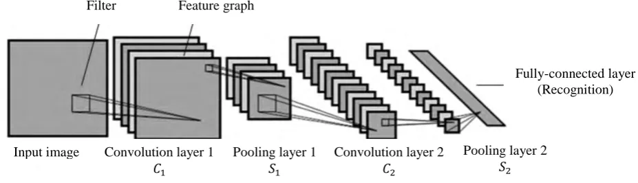
Figure 1. Convolutional Neural Network. Input image

𝐶1

Convolution layer 1

𝐶2

Convolution layer 2

𝑆1

Pooling layer 1

𝑆2

Pooling layer 2 Filter Feature graph

Assume the input training dataset of the CNN has N images, each of size 𝑚 × 𝑛, and the size of convolution filter is 𝑘₁× 𝑘₂. For the 𝑖𝑡ℎimage 𝐼_𝑖 , denote all the image blocks of size 𝑘₁ × 𝑘₂in it by

𝑥_𝑖1, 𝑥_𝑖2, … , 𝑥_{𝑖(𝑚𝑛)} ∈ 𝑅𝑘1𝑘2_{, where} 𝑥

𝑖𝑗represents the 𝑗𝑡ℎimage block in 𝐼𝑖 . Then remove the mean value for

each 𝑥_𝑖𝑗 and get the image block data of 𝐼_𝑖, 𝑋̅_𝑖 = [𝑥̅_𝑖1, 𝑥̅_𝑖2, … , 𝑥̅_{𝑖(𝑚𝑛)}]. In this way, we can get the training image dataset

𝑿 = [𝑋̅1, 𝑋̅2, … , 𝑋̅𝑁] ∈ 𝑅𝑘1𝑘2×𝑁𝑚𝑛(1)

Then, this work obtains the eigenvector by using PCA to minimize the reconstruction error, as the following equation:

𝑚𝑖𝑛_𝑽∈𝑅𝑘1𝑘2×𝐿||𝑿 − 𝑉𝑉𝑇||_𝐹𝟐 𝑠. 𝑡. 𝑉𝑇𝑉 = 𝑰𝐿, (2)

where𝑰𝐿is an 𝐿 × 𝐿 identity matrix. 𝑉is composed of the first 𝐿 smallest eigenvectors of the covariance

matrix 𝑿𝑿𝑇, and of size 𝑘₁𝑘₂× 𝐿. So V represents the primary component of the input image dataset. And then the filter set 𝑊′= [𝑊₁′, 𝑊₂′, … , 𝑊_𝐿′], which is learned by PCA and used to initialize the network, is as following equation:

𝑊_𝑙′_{= 𝑚}

𝑘1𝑘2(𝑞𝑙(𝑿𝑿𝑇)) ∈ 𝑅𝑘1𝑘2, 𝑙 = 1,2, … , 𝐿,(3)

where𝑚_k1k2(𝑣)is the mapping from vector 𝑣 ∈ 𝑅𝑘1𝑘2_{to matrix} 𝑊 ∈ 𝑅𝑘1𝑘2_{, and} 𝑞

𝑙(𝑿𝑿𝑇)refers to the

𝑙th_{smallest eigenvector of 𝑿𝑿}𝑇_.

The primary components of the local image blocks of the training data, obtained by PCA, can represent the local features of data to the greatest degree. Besides, as filters, they can obtain the main information about local features, and the change and difference between these features. Therefore, using PCA to train filters can be regarded as a simple Autoencoder.

B.Concolutional Neural Network

As shown in Figure 1, a traditional CNN is composed of convolution layers, pooling layers and fully-connected layers.In the convolution layers, feature graphs can be obtained by convolving the input image with the filter and passing through an activation function. Then they are obscured and generalized in the pooling layers. Finally, the fully-connected layers output the features, which are used to recognize images.

The formula of the output of a convolution layer is as Equation (4).

𝑥_𝑗(𝑙) = 𝑓(∑_{𝑖∈𝑀𝑗}𝑥_𝑖(𝑙−1)∗ 𝑤_𝑖𝑗(𝑙)+ 𝑏_𝑗(𝑙)), (4)

where ‘* ’ refers to the convolution operation. In the 𝑙𝑡ℎlayer, 𝑤_𝑖𝑗(𝑙)is the weight from 𝑖𝑡ℎinput to

𝑗𝑡ℎ_{neuron, and 𝑥} 𝑗

(𝑙)

and w_ij(l)are the output and bias of the jthneuron. f is the nonlinear activation function.

Another difference between the traditional CNN and the algorithm proposed in this paper is that a local contrast normalization operation is added after convolution. The formula of this operation is as Equation(5), and it is proved to be able to improve the feature invariance and increase the sparsity and robustness of the model to raise the recognition rate.

x_ij(l) =xi,j(l−1)−mN(i,j)(l−1)

σ_N(i,j)(l−1) , (5)

wherex_i,j(l−1)corresponds to the feature in location (i, j) in the (l − 1)thlayer. x_ij(l)is the output value after

normalization. m_N(i,j)(l−1)andσ_N(i,j)(l−1)are the mean and variance of local region N(i, j).

After normalization, it is downsampling. In order to preserve the information to the maximum extent while ensuring the feature invariance, and get better robustness and higher recognition rate, I use the maximum probability sampling method. The sampling value P_αonly response when there is at least one neuron is on. Otherwise, P_αdoes not response. This can be expressed as Equation (6).

P(P_α= 1|x) = ∑i,j∈Bαexp (Wk∗x)ij+bk

1+∑ exp (Wk_∗x)ij+bk

i,j∈Bα (6)

C.PCA Unsupervised Training Target Recognition Algorithm

Based on the CNN model and the PCA unsupervised training method mentioned above, Figure 3 shows the flow diagram of the vision-based CNN target recognition algorithm.

Algorithm

Step1. Train the filters:

(a) Find all the image blocks of size 𝑘₁× 𝑘₂ in the training images, and construct dataset 𝑿 using Equation 1.

(b) According to Equation 2, get the initial filter weight of CNN from 𝑿 , using PCA unsupervised training.

Step2. Calculate the feature graph 𝑥(1)after convolution layer and the activation function, using Equation 4.

Step3.Operate local contrast normalization on x(1), and denote the output as 𝑥(2).

Step4.Obscure and generalize 𝑥(2)using maximum probability sampling, and get 𝑥(3).

Step5.Repeat Steps 1-4 with 𝑥(3)as input dataset. Denote the output feature graph as 𝑥(4).

Step6. Merge 𝑥(4)as a column vector, which is the input of the fully-connected layer. Usesoftmax classifier

to get the recognition result.

Step7. Calculate the difference between the results and tags, and use the back propagationmethod[10] to

adjust weight from top to down.

EXPERIMENTS & RESULTS

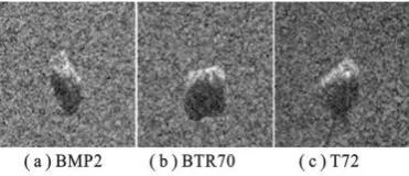
The simulation experiment uses moving and stationary target acquisition and recognition (MSTAR) dataset, which is composed of the ground stationary military target data measured by SAR. Three types of SAR targets are used in the experiment: BMP2 (armored vehicle), BTR70 (armored vehicle), T72 (main battle tank), which are all shown in Figure 4. The image resolution is 0.3m×0.3m, of size 128m×128m, and the azimuth coverage range is 0°～360°. The training set has 698 target images with a 15° depression angle,

and the test set has 1365 target images with a 17° depression angle. Since the corrected target are basically in the center part of each image, the central 90m×90m block of the image is taken as the experimental data. And then preprocess the data to reduce the impact of background on feature extraction and target recognition. The reason for choosing MSTAR database is that there are few labeled training data in it, which can reflect the superiority of the unsupervised pre-training algorithm. In the experiment, the central processing unit (CPU) is 2.8GHz with memory of 3GB, and it is performed in Matlab2010b environment.

A.Comparison Test of the Algorithm Recognition Rate

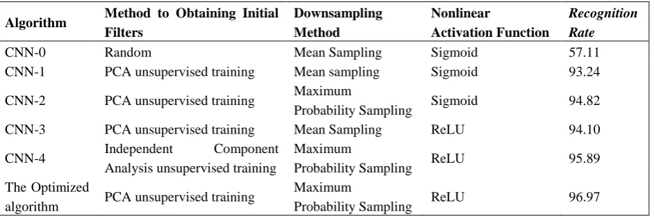
The model of the CNN proposed in this paper is in Figure 1, and it operates as the flow diagram in Figure 5. The network is composed of 5 layers: two convolution layers, two pooling layers (down sampling layer) and one fully-connected layer. There are 8 filters in layer 1, 16 in layer 2, whose size are all 7×7. The slide sizes in the pooling layers are both 2, and it use maximum probability sampling method. During the experiment, I compare the network with other five CNNs, whose details and performance are all shown in Table 1.

As can be seem from Table1, for MSTAR data, the recognition rate of the optimized algorithm this work proposed is obviously improved, compared with those of the CNNs under different conditions. The convolution filters are the core that affects the recognition rate of a CNN. The training is actually the adjustment of its filters and the extracted features of each layer. Since these features are used for classification and identification, the adjustment is quite important. The recognition rate of CNN-0 is very low because the initial filters are generated by random. In this way, the network can easily reach a local optimum, but not global optimum, when the image background is relatively complex, or the data size is very small. So it is very difficult or unable for such networks to obtain suitable convolution filters through training. PCA can properly obtain a set of bases for the linear combination of all data in the input dataset, which can represent the local feature information of the input training image to the largest extent. Using this set of bases as filters can better extract the most primary component of local features, and the change and difference among the features from original data. Therefore, CNN-1 can avoid local optimum and solve the problem of whether CNN can recognize MSTAR or not.

Compared with CNN-1, CNN-2 and CNN-3 have certain improvements in their recognition rate. By maximizing the probability, the sampling method and preserve the feature information to greatest extent while guaranteeing the invariance. The ReLU function can efficiently avoid local optimum and overfitting, and improve the training speed.

The optimized algorithm has a higher recognition rate relative to CNN-4. The reason is that, compared with independent component analysis, PCA can obtain better filters from the input dataand has better robustness and self-adaptability.

TABLE I. DETAILS AND RESULTS OF THE COMPARISON TEST.

Algorithm Method to Obtaining Initial Filters Downsampling Method Nonlinear Activation Function Recognition Rate

CNN-0 Random Mean Sampling Sigmoid 57.11 CNN-1 PCA unsupervised training Mean sampling Sigmoid 93.24

CNN-2 PCA unsupervised training Maximum

Probability Sampling Sigmoid 94.82 CNN-3 PCA unsupervised training Mean Sampling ReLU 94.10

CNN-4 Independent Component Analysis unsupervised training

Maximum

Probability Sampling ReLU 95.89 The Optimized

algorithm PCA unsupervised training

Maximum

Probability Sampling ReLU 96.97

B.Algorithm Robustness Experiment

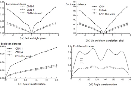
In order to verify the robustness of this network, the experiment uses different types of images after translation, scale and rotation transformation. Then the Euclidean distances of the output features of the fully-connected layer, both before and after the transformation, are calculated and used to measure the robustness of the output features to the target transformation. The less the distances changes, the less sensitive the features are to transformation, so the better the robustness is. The experiment is conducted on any selected image in MSTAR dataset, and compares the proposed network with CNN-1 and CNN-4. The test results are all shown in Figure 5.

since slight change in one image can cause great change in its features. The better robustness of this proposed algorithm firstly comes from the PCA unsupervised training method, from which filters are obtained to extract the most primary component in local features, the change and difference among features of data. Secondly the maximum probability down sampling method and choosing the ReLU function also contributes. This preserves the feature information to the largest extent while guaranteeing the variance and efficiently avoiding reaching a local optimum. Finally, the algorithm uses local contrast normalization, which improves the robustness of the target images with noise in the dataset.

Figure 5. Robustness Experimental Results.

CONCLUSIONS

REFERENCES

1. Dan, Cireşan, and U. Meier. "Multi-Column Deep Neural Networks for offline handwritten Chinese character classification." International Joint Conference on Neural Networks IEEE, 2015:1-6.

2. Osendorfer, Christian, H. Soyer, and P. V. D. Smagt. Image Super-Resolution with Fast Approximate Convolutional Sparse Coding. Neural Information Processing. Springer International Publishing, 2014:250-257.

3. Roth, S., and U. Schmidt. "Learning rotation-aware features: From invariant priors to equivariant descriptors." Computer Vision and Pattern Recognition IEEE, 2012:2050-2057.

4. Ozeki, Makoto, and T. Okatani. Understanding Convolutional Neural Networks in Terms of Category-Level Attributes. Computer Vision -- ACCV 2014. Springer International Publishing, 2015:362-375.

5. Burges, Christopher J. C, J. C. Platt, and S. Jana. "Distortion discriminant analysis for audio fingerprinting." Speech & Audio Processing IEEE Transactions on 11.3(2003):165-174.

6. Lécun, Yann, et al. "Gradient-based learning applied to document recognition." Proceedings of the IEEE 86.11(1998):2278-2324.

7. Nebauer, C. "Evaluation of convolutional neural networks for visual recognition." IEEE Trans Neural Netw 9.4(1998):685-696.

8. Jarrett, Kevin, et al. "What is the Best Multi-Stage Architecture for Object Recognition?." 30.2(2009):2146-2153.

9. Browne, Matthew, and S. S. Ghidary. "Convolutional Neural Networks for Image Processing: An Application in Robot Vision." Ai 2003: Advances in Artificial Intelligence, Australian Conference on Artificial Intelligence, Perth, Australia, December 3-5, 2003, Proceedings DBLP, 2003:641-652.

10. Jarrett K, Kavukcuoglu K, Ranzato M A, et al. What is the Best Multi-stage for Object Architecture?[C]// Proceedings of the IEEE 12th International Conference on Computer Vision. Piscataway: IEEE, 2009:2146-2153.