Microphone wind noise reduction using singular spectrum analysis techniques

singular spectrum analysis techniques

Eldwaik, O and Li, FF

Title

Microphone wind noise reduction using singular spectrum analysis 

techniques

Authors

Eldwaik, O and Li, FF

Type

Conference or Workshop Item

URL

This version is available at: http://usir.salford.ac.uk/id/eprint/44787/

Published Date

2017

USIR is a digital collection of the research output of the University of Salford. Where copyright 

permits, full text material held in the repository is made freely available online and can be read, 

downloaded and copied for non­commercial private study or research purposes. Please check the 

manuscript for any further copyright restrictions.

Vol. 39. Pt. 1. 2017

MICROPHONE

WIND

NOISE

REDUCTION

USING

SINGULAR SPECTRUM ANALYSIS TECHNIQUES

Omar Eldwaik School of Computing, Science & Engineering, Acoustics Research Centre, University of Salford, Manchester, UK

Francis F. Li School of Computing, Science & Engineering, Acoustics Research Centre, University of Salford, Manchester, UK

1

INTRODUCTION

Recent and rapidly increasing innovation in acoustic sensing technology and Internet of Things (IoT) motivated the use of sound signatures to identify objects, sense the environmental variables and capture relevant events. Besides to common scenarios of audio recording, acoustic sensing assists daily activities, industrial operations and environmental management in many ways, including environmental noise and soundscapes monitoring. Outdoor acoustic sensing is particularly challenging as the transducers, typically microphones, are exposed to adverse weather conditions such as rain and wind; these might induce extraordinary noises in microphone signals. The ever increasing research activities and demand of acoustic sensing in environmental sounds and soundscapes monitoring along with the hugely untapped potentials of acoustic sensing for added-value applications have driven the interest of this study.

Wind noise is a known problem that contaminates microphone signals in many field measurement and audio recording scenarios. Wind induced noise from microphone signals causes many problems in the subsequent use of acoustic information; and this is one of the major problems in acoustic sensing in environmental noise and soundscapes monitoring applications. Wind noise problem is also an unsolved one in audio recording outdoor, such as field news broadcasting.

In audio recorded outdoor media applications, microphone wind noise is unpleasant nuisance. The problem can become more severe in acoustic sensing for environmental sounds and soundscapes monitoring and even smart environments, applications: malfunctions can happen. For environmental sound monitoring, microphone wind noise contaminates and alters the soundscapes to be monitored, since the microphone noise is not what human listeners normally hear in the windy conditions, but the noise induced by the interaction between the wind and the microphones. For this reason, in this paper the terminology “microphone wind noise” and/or “wind noise in microphone signals” are used instead of wind noise to highlight that the noise of concern is induced by the presence of a microphone in windy conditions, and such noise appears in the microphone signals.

The current paper represents a new approach to the wind noise problem. Instead of filtering, a separation technique is developed. Signals are separated into wanted sounds of specific interest and wind noise, with reduced distortion imposed on the wanted signals, based on the statistical feature of wind noise. The new technique is based on the so called Singular Spectrum Analysis (SSA) method, which has been recently seen many successful paradigms in the separation of biomedical signals, e.g. separating heart sound from lung noise. It has also been successfully implemented to de-noise signals in many various applications.

Vol. 39. Pt. 1. 2017

2

BACKGROUND

Outdoor acoustic sensing can be applied to collect data in bioacoustics data analysis, monitoring pollution along with some of the pioneering applications that impact inhabitants’ daily lives such as surveillance type of applications1_{. For example, in bioacoustics data analysis, scientists who are} interested in environment changes monitoring and birds’ chirps, which are of the interest outdoor sound sensing, will rely on deploying various types of acoustic sensors in the field. Distance outdoor microphones could help ecologists record whatever sound they want instead of conducting standard surveys. Although such method will bring some advantages over classical surveys, such as saving time and efforts, providing continuous recordings, and could scale over long period and huge area, but the data collected will include much of background noise that makes annotation of bird vocalisations more difficult. And hence, it is to consider microphone wind noise as a serious problem that affects the sensed data2_.

For environmental noise level measurement, especially long term measurement or monitoring, microphone wind noise is added to the recorded noise level, giving inaccurate results. Wind shields are commonly used on microphones in outdoor sound acquisition to prevent the wind from exciting the membrane of the microphone; however the effectiveness is limited, residual microphone wind noise remains problematic. Moreover, with the fast development and use of small and smart high-technological consumer products like hearing aids along with the introduction of smart city paradigm that based on applying acoustic sensing technology; every-day experience for people around the world has widely increased nevertheless what the weather condition is. However, to deal with microphone wind noises that interfere with the signals of interest, a large number of standard or common approaches ranging from fixed, optimal to adaptive filtering have been applied to mitigate wind noise in microphone signals. Due to the broadband and time varying nature of microphone wind noise, such general noise suppression algorithms show some but limited effectiveness. Contemporary and powerful signal processing methods are sought to address the wind noise issues and can yield better results, e.g3_.

Many attempts were made in the past using various filtering techniques to broadband noise suppression. These methods worked to some extent, but have intrinsic limitations of distorting wanted signals and difficulties in retaining accurate signal energy levels to meet the measurement requirements. However, when the wind noise is removed, wanted signals are distorted considerably. For event detection or decision making from acoustic signatures, distorted signals cause errors or mis-judgements, mitigating the reliability, usability or even safety of such systems. Linear separation in subspace seems to be potential solution to circumvent these problems.

3

WIND NOISE PROBLEM IN OUTDOOR MICROPHONE

SIGNALS

In environmental noise and soundscapes monitoring, environmental sounds are such a rich source of acoustic data, and at the same time they comprise much background noise, which hinder the extraction of useful information4_{. Environmental sounds are highly considered as non-stationary and} underexploited source of data. Having difficulties in describing such sounds using common audio features as well as defining appropriate features for environmental sounds in automatic acoustic classification systems, is an issue of concern. There is a variety of environmental sound sources that produce different forms of sound. These environmental sources produce unwanted sounds which considered as noise sources5_{. The heavy presence of environmental noise such as wind} covers useful information and limits the usage of such data source efficiently to extract semantic information.

Vol. 39. Pt. 1. 2017

has an adverse effect on the perceived quality of the target sensed sound and posing difficulties to properly distinguish the sensed or recorded event of interest. Meanwhile, the performance of other processing algorithms such as speech or speaker recognition may also be affected6_.

For many decades, noise reduction algorithms have been developed and applied to suppress undesired components of a signal or at least to mitigate the impact of such components, which considered as noise, on the signal of interest. Generally, the removal of noise is notan easy task as the problem is manifold, many unsolved issues owing to the different environmental sound sources that produce noise and particularly microphone wind noise. Wind noise is highly non-stationary in time and even sometimes it resembles transient noise which makes it hard for an algorithm to estimate the noise from a noisy signal.

Turbulent airflow over the microphone casing and membrane causes wind noise which considered as a particular type of acoustic interference that creates an acoustic effect of a relatively high signal level6_{. The turbulence generated by the interaction of the wind and the microphone along with the} fluctuations that occur naturally in the wind are the two components of wind noise6_{. Wind noise} fluctuates rapidly and wind gusts might have very high energy3_{. The spectrum of the recorded wind} noise has been described as a broadband but decreasing function of frequency, showing the bulk of the energy in the lower region of the spectrum6_.

Microphone wind noise leads to listener fatigue as it is often annoying. It is impulsive and non-stationary in nature with high amplitude that may exceed the nominal amplitude of the signal of interest. Due to that, conventional noise reduction schemes, such as spectral subtraction or statistical-based estimators, cannot effectively attenuate wind noise7_{. Additionally, traditional} remedy for wind noise compromises the quality of the sensed acoustic data. Wiener filter method for example, which is arguably one of the most well-established random noise optimal removal filters used for removing noise from a signal when the signal of interest and the noise have different frequency characteristics, shows some but limited performance3_{. Methods that make use of two or} more sensors known as multi-microphone and microphone array are relatively considered effective for reducing wind noise as the difference in propagation delay between wind and acoustic waves can be exploited6_{. However, the difficulty and high cost in deploying these complicated setups limit} their prevalent use. Single-microphone wind-noise reduction is still an open ended problem and a technical challenge for further extensive research.

The main concern discussed in this paper is the destructive impact on the wanted sensed signals. Moreover, one of the greatest challenges for the future digital ecosystem is to better reduce such unwanted environmental noise in outdoor acoustic monitoring. Hence, improving de-noising techniques or implementing new techniques that may lead to better solutions and be effective alternatives to the classic methods become increasingly important against the harmful effect of wind on the perceptual quality of the wanted signals.

While the objective of the present investigation focuses on microphone wind noise reduction in the context of environmental noise management and soundscapes monitoring, the current study attempts to cover certain important aspects and develops a more rigorous understanding of the SSA technique as a proposed method in this paper.

4

RATIONALE

Vol. 39. Pt. 1. 2017

The SSA is a model free and nonparametric technique for time series analysis works with arbitrary stochastic processes such as linear or nonlinear, stationary or stationary, and Gaussian or non-Gaussian without specific assumptions or restrictions. The end results and effectiveness may differ depending upon the suitably determined window lengths and separability of the dataset itself in the singular spectral domain9,10,11_.

As the SSA method decomposes a time series into its singular spectral domain components, which are physically meaningful in terms of oscillatory components and trends and reconstructs the series by leaving the random noise component behind, such fundamentals give it a great advantage for noise reduction12_{. Furthermore, and unlike many other methods, the SSA works well even for small} sample sizes9_{, making it possible to quickly update the coordinator rotation to varying signals block} by block in relatively small blocks.

The SSA is an effective method that can be used for solving many problems such as finding trends of different resolution, smoothing, extraction of seasonality components, extraction of periodicities with varying amplitudes, simultaneous extraction of complex trends and periodicities, finding structure in short time series, etc. The basic capabilities of the SSA can lead to solve all these problems. When compared with other time series analysis methods, it shows certain superiority, potentials and broader application areas, and competes with more standard methods in the area of nonlinear time series analysis11_.

As a method of prediction and forecasting specially for real time series that usually has a complex structure, the SSA shows potential capabilities because it is not sensitive to the dynamical variations as well as non-parametric which makes no prior assumptions about the data10_{. A great} deal of research work has been conducted on the SSA to consider it as a de-noising method12_{. The} SSA technique has also been applied for extracting information from noisy dataset for biomedical engineering and other applications13_{. The method has been employed and shown its capabilities for} noise reduction for longitudinal measurements14_{.The superiority of the SSA over other methods in} biomechanical analysis was clearly demonstrated by several examples presented in the work in15_.

In recent years, traditional methods applied for time series analysis such as power spectra have been augmented by new methods. As an alternative to traditional digital filtering approaches, the SSA is presented in many applications. The SSA is introduced in a wide range of applications as a de-noising and raw signal smoothing method. It is mainly based on principles of multivariate statistics15_{. Basically, a number of additive time series can be obtained by decomposing the original} time series to identify which of the new produced additive time series be part of the modulated signal, and which be part of random noise15_{. It is showed in}8 _{that using the SSA for data} pre-processing is a helpful procedure that encourages improving the results of any time series for data mining, and many future environmental studies can probably adapt such studied approaches.

The SSA decomposes time series and allows for meaningful grouping of these components in a linear manner in the subspaces. It is therefore thought that if the dataset is separatable to wind noise and the wanted signals, and the proper grouping method can be identified, wind noise can be separated. Since the SSA is non-model based, in other words it is data driven. Empirical methods are needed to identify its applicability for specific problems. Following an outline of the SSA method, empirical study is carried out in this paper to experimentally investigate and show how the SSA can separate microphone wind noise by establishing a framework and creating a testing platform to perform different experiments.

5

THE METHOD

5.1 The SSA Theory

The term “singular spectrum” came from the spectral (eigenvalue) decomposition of a given matrix

Vol. 39. Pt. 1. 2017

specific numbers that make the matrix

A





I

singular when the determinant of this matrix is equal to zero. In this mathematical illustration, matrix

I

is the identity matrix. Singular spectrum analysis, per se, is, the analysis of time series using the singular spectrum. Therefore, the time series under investigation needs to be embedded in a so-called trajectory matrix as detailed in the sub section below and many basic operations of the SSA algorithm are elementary linear algebra16_.

The SSA method provides a representation of a time series in the so-called Eigen domain in terms of eigenvalues and eigenvectors of a matrix constructed from the time series17,18_{. The aim is to} make a decomposition of the original time series into a small number of independent and interpretable components such as; a slowly varying trend, oscillatory components (harmonics) and a structure less noise. Once the SSA decomposes signals in the Eigen-spaces, it selects and groups the principle components according to their contributions. Eventually the SSA reconstructs the wanted components back to the time domain. The reconstruction of the original time series is accomplished by using estimated trend and harmonic components19_.

In principal, the idea of the SSA is to embed a time series

X

(

t

)

into multi-dimensional Euclidean space and find a subspace corresponding to the sought-for component as a first stage. The second stage is to reconstruct a time series component corresponding to this subspace. At the first decomposition stage, the time series is decomposed into mutually orthogonal components after computing the covariance matrix from the constructed trajectory matrix. The covariance matrix is needed to compute the eigenvalues and their associated eigenvectors and further the principle components. In the reconstruction stage or also known as estimation stage, the time series is reconstructed by selecting those components that reduce the noise in the series20_.

The key element in the de-nosing process is to remove the noise without losing a significant portion of the signal and this can be accomplished with the SSA. De-noising using the SSA is sometimes referring to as data adaptive16_{. The SSA can provide an important concept from the time series} which known as statistical dimension. The statistical dimension of the process from which the time series was taken is defined as the number of eigenvalues before the noise floor. This concept develops the use of the SSA as a de-noising technique16_{. A rough estimate of the number of} degrees of freedom needed to describe the dynamical system represented by the record can be given using this concept. The main aspect in studying the properties of this method is to identify the suitable window length and how well different components can be separated from each other10_.

5.2 The SSA Algorithm

A short description of the SSA algorithm can be outlined in several steps as follows;

1) Constructing the so-called trajectory matrix: in this step we transfer a one-dimensional time series into the multi-dimensional series considering that the single parameter of the embedding is the window length.

A one-dimensional time series shown in (1) can be transferred into a multi-dimensional series in the embedding step which can be viewed as a mapping process.

t N

X

X

X

t

X

(

)



₁

,

₂

,...

(1)

The multi-dimensional series contains vectors

v

k which called m-lagged vectors (or, simply, lagged

vectors).

)

...,

,

(

_{1 2 (  1)}



_{k k k N m} T

k

x

x

x

t

v

(2)

where m is the window length,

N

_t is the length of the time series and k is the lag (or delay shift) given as in (3)

1

,...,

1

,

0





m

k

(3)

The number of rows in the resultant matrix that can be filled with the values of

X

(

t

)

after the transformation to multi-dimensional series considering the lag k is given by

1







N

m

Vol. 39. Pt. 1. 2017

In this step, the single parameter is the window length m which is an integer such that

2



m



N

_t. The result of the embedding process is a matrix Y with entries

(

x

_ij

)

_iN_,,_jm_1. Matrix Y is called the trajectory matrix and it is a Hankel matrix (i.e. all the elements along the diagonal

i



j



const

are equal).

Y



[

v

k0

,....,

v

km1

]

(5)

2) Computing the covariance matrix: the covariance matrix can be estimated directly from the data and is considered as a Toeplitz matrix with constant diagonals. The covariance which referred to as correlation in engineering can be computed using a MATLAB function specified by “cov” that gives a vector of size m as a first method. The covariance between

X

(

t

)

and

X

(

t



k

)

with values of k as in (3) is represented in this vector. The values in this vector will be used to construct the diagonal-constant matrix. The covariance matrix is denoted by C and of dimension m × m. The entries

c

_ijof this matrix depend only on the lag

i



j

as in (6) 19_.

1

(

)

(

)

1



 













N i j

t t

ij

t

j

i

t

X

t

X

j

i

N

c

(6)

where

N

_t represents the number of data points, the entries

c

_ijwhen

i



j



0

for

i



j

, are the entries across the main diagonal, that is, their values typically tend to be close to 1. This step is the preparation for applying singular value decomposition (SVD). The covariance matrix can also be computed, as a second method, using the trajectory matrix and its transpose by

Y

Y

C



T (7)

3) SVD of the covariance matrix: it is a step of computing the diagonal values and their corresponding vectors where each presented in a separate matrix. The first is a diagonal matrix of the ordered eigenvalues and the second is the corresponding orthogonal matrix of the eigenvectors. Performing the singular value decomposition of the trajectory matrix can be obtained via the eigenvalues and eigenvectors of the covariance matrix. The eigenvalue decomposition of the covariance matrix is given by

T

C









(8)

The resultant matrices are the eigenvalues aligned in the matrix Lambda

(



)

and their associated eigenvectors presented in the matrix RHO

(



)

. The eigenvectors matrix consists of a set of vectors

in the form

e



[

e

k_j

]

that represents the jth _{component of the k}th _{eigenvector in the matrix RHO}

with

j



1

,...,

N

, and

k



1

,...,

m

. For more clarification the first vector is

e

₁T



[

e

1_j

,...,

e

1_N

]

, the

second is

e

₂T



[

e

2_j

,...,

e

_N2

]

, and so on up to

k



m

. The spectral decomposition of the covariance

matrix yields the diagonal eigenvalues matrix



considering that the ith _{column of RHO is the}

eigenvector corresponding to the eigenvalue in the ith _{column of}



_{. Matrix}



_{is symmetric with}

entries



_i along the leading diagonal for

i



1

,...,

m

.

4) Computing the principle components: this step is to select a group of eigenvectors that associated to the most dominant eigenvalues. In this grouping step, the matrix U of principle components (PCs) is introduced as the projection of the embedded time series onto the eigenvectorswhen considering the normalization, and hence it becomes



Y

m

U



1

(9)

Vol. 39. Pt. 1. 2017

embedded time series introduced in the trajectory matrix and ordered in the same way as the eigenvectors. Selecting the principle components that correspond to the significant eigenvectors associated to the larger eigenvalues is one kind of grouping which used to exclude components that mainly represent noise such those associated to the lower eigenvalues. The selected groups of the principle components are presented in vectors and can be aligned in a matrix denoted by Z and constructed in a similar way of the trajectory matrix Y with opposite direction. This kind of grouping will help in reconstructing the time series by computing the reconstructed components.

5) Reconstruction of the one-dimensional series: this step is to compute the reconstructed component matrices. The reconstruction components (RCs) can be computed by projecting the principle components presented in the matrix Z back onto the eigenvectors of matrix RHO when the normalization is considered and hence



Z

m

RCs



1

(10)

The RCs for the original input can be determined by averaging along anti-diagonals (this is known as diagonal averaging).The RCs can also be calculated by inverting the projecting principle components;

U



Y



onto the eigenvectors transpose matrix

T T

U

Y

RCs









(11)

6

EXPERIMENTS AND RESULTS

6.1 Description of Experiments

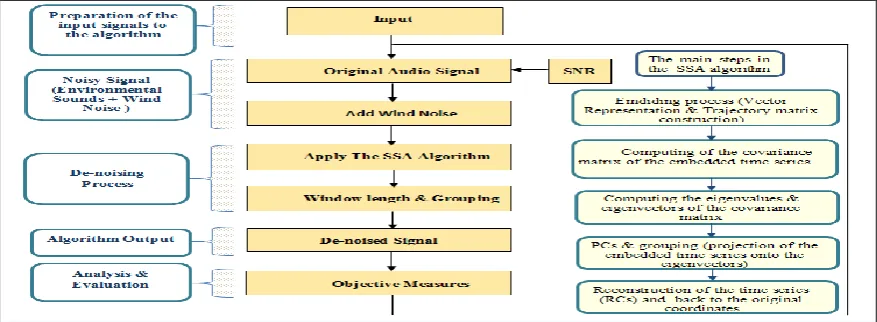
A range of experiments were carried out to identify the potential and capability of the SSA in wind noise reduction. Experiments started with separation of wind noise from deterministic signals such as sine, triangular waves and their mixtures and moved to sweep tones and environmental sounds, particularly birds’ call. Although in call cases, notable wind noise reduction was observed, results are different from case to case due to the complexity of the environmental sounds. Due to the page limitation for a conference contribution, only results from separation of outdoor wind noise from birds’ chirps are detailed in the current paper. The experimental procedure of the SSA method is shown in Figure 1. The experiments were carried out on MATLAB platform.

[image:8.595.77.516.520.681.2]

Figure 1. A flowchart of the experimental procedure

The algorithm generates a trajectory matrix Y from the original time series X(t) by sliding a window of length m. Window length is an integer such that

2



m



N

_t.

It has been recommended that m should be large enough but not greater thanNt 2. If m is too

Vol. 39. Pt. 1. 2017

variables. Generally, large values of m induce longer period oscillations to be resolved. In spite of the considerable attempts and various methods that have been considered for choosing the optimal value of the window length, there is inadequate theoretical justification for such selection20_{. As a} common practice, however, the window length can be computed as

t

N 4

1 16_.

The trajectory matrix is approximated using SVD. The covariance matrix which constructed by performing matrix operations is required for computing the eigenvalues and eigenvectors. The eigenvalues of C are presented along the main diagonal of a square matrix. Determining the eigenvalues in this way is known as Singular Value Decomposition. Their associated eigenvectors, which also presented in a square matrix, are needed to compute the principle components as they represent the axes of projection.

The first eigenvectors represent a high-frequency oscillation if we consider successive elements of the eigenvectors over time, while the rest capture the lower-frequency components of the time series. The components to be used to reconstruct the series must be properly chosen based on the singular spectrum appearance. The principle components can be computed by projecting the trajectory matrix Y onto the eigenvectors. Up to this step, the representation of our signal is still in the Eigen domain. Therefore, the principle components are incomparable to the original time series. The principle components should be selected in identified groups to compute the reconstructed components. The last step, however, is to reconstruct the series from the approximated trajectory matrix. The output of this step is the Singular Spectrum of the original time series which must be a column vector represents the eigenvalues.

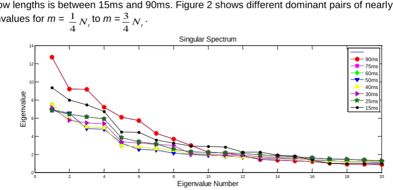
6.2 Window Length Optimisation

In order to optimise the window length, we calculate singular spectra for our record using eight different window lengths. In our experiments, we selected a sample of 60 seconds of our audio recordings of birds’ chirps using an average of a frame size of 100ms. The selected range of the window lengths is between 15ms and 90ms. Figure 2 shows different dominant pairs of nearly equal eigenvalues for m =

t

N 4

1 _{to m =}

t

N 4

3 _.

0 2 4 6 8 10 12 14 16 18 20

0 2 4 6 8 10 12 14

Singular Spectrum

Eigenvalue Number

E

ig

e

n

va

lu

e

[image:9.595.100.492.438.628.2]

90ms 75ms 60ms 50ms 40ms 30ms 25ms 15ms

Figure 2. Window length optimisation

A clear break between these singular values and the others, which spread out in a nearly flat noise floor, can also be realised. For the window length above and below this band, indifferent eigenvalues are obtained. For example, for m=

0

.

25

N

_tas illustrated in the figure, two dominant pairs of nearly equal eigenvalues can be seen. Thus, the statistical dimension (

d

_s) = 4 for

m=

0

.

25

N

_tseems to be the most dominant value in this example since the record is the superposition of oscillations perturbed by wind noise. It has been theoretically shown, however, that

Vol. 39. Pt. 1. 2017

It is worthwhile mentioning that such equality between the eigenvalues should be considered as an important aspect in the grouping criteria. Consequently, any unequal location of the singular values of the pair itself over the threshold and in comparison with the next pairs will indicate that the eigenvalues have different frequencies and in turn different contribution. Therefore, for a proper grouping, the eigenvalues should have the same contribution as the eigenvalues pairs are considered dominant in terms of equality. Dominant eigenvalues in the singular spectrum correspond to an important oscillation of the system for each pair of nearly equal as remarked in16_.

6.3 Results

Figure 2 shows the eigenvalues from a decomposed signal corrupted with wind noise arranged in descending order. Only first few of them carry large amount of energy. The first pairs of eigenvalues, however, are the ones with less correlation. The high correlation ones are those which left behind and generally represent the noise.

In this paper, the grouping was performed based on the best selection of the most dominant pairs of the eigenvalues. It is worth to mention that the number of such dominant eigenvalues differs as long as the window length changes.

0 500 1000 1500 2000 2500 3000 3500 4000 4500 -1.5 -1 -0.5 0 0.5 1 1.5x 10

-5

Data point

The first two leading pairs of the principle components

A m p li tu d e

Original noisy record Reconstructed series

0 500 1000 1500 2000 2500 3000 3500 4000 4500 -1.5 -1 -0.5 0 0.5 1 1.5x 10

-5

Data point The third pair of the principle components

A m p li t u d e

Original noisy record Reconstructed series

0 500 1000 1500 2000 2500 3000 3500 4000 4500 -1.5 -1 -0.5 0 0.5 1 1.5x 10

-5

Data point The fourth pair of the principle components

A m p li tu d e

Original noisy record Reconstructed series

0 500 1000 1500 2000 2500 3000 3500 -6 -4 -2 0 2 4 6 8x 10

-5 Original noisy signal

[image:10.595.95.503.340.594.2]

Data point A m p li tu d e

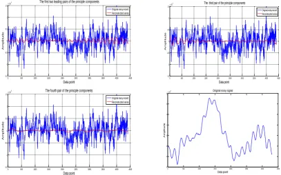
Figure 3. The leading four principle components used for grouping and reconstruction

In our example (with m =

0

.

25

N

_t) as shown in Figure 3 we see that, indeed, the first two pairs of eigenvectors correspond to important oscillations and our signal can be reconstructed based on the selection of these two pairs in the grouping step. The phases are in quadrature and regular changes in amplitude are obviously present for the first two pairs of eigenvectors. In contrast, for the third and fourth pairs, there is slight coherent phase relationship between their two eigenvectors. However, the eigenvalues associated with these pairs are mostly located in the noise floor of the singular spectra as they are of low variance.

Vol. 39. Pt. 1. 2017

principal components, which are noisy with low amplitudes. The grouping therefore has been performed in this way as it has been experimentally found that selecting lower eigenvalues beyond the “elbow” point shown in the singular spectra will only produce noisy signals. Eventually, projecting the principle components onto the orthogonal matrix of the eigenvectors produces the reconstructed components of our record.

0 500 1000 1500 2000 2500 3000 3500 4000 4500

-5 0 5x 10

-6

Data point

Noisy and reconstructed series with the residual noise

A m p li tu d

e Original noisy signal_{Reconstructed series}

0 500 1000 1500 2000 2500 3000 3500 4000 4500

-5 0 5x 10

[image:11.595.117.482.178.314.2]

-6 Data point Residual series M a g n it u d e

[image:11.595.112.482.420.718.2]

Figure 4. Reconstructed series vs original noisy signal and residual series

Figure 4 illustrates a comparison of the noisy record, which is a mixture of our signal of interest (bird chirps and wind noise), with the reconstructed one (filtered). The differences between reconstructed series and original noisy signal are highlighted in the top part of the figure. It is clear from the bottom of the figure, a considerable amount of noise (denoted as residual series) was separated out. However, the findings revealed that the de-noised signal resembles the clean one. As seen above, the SSA canreadily extract and reconstruct periodic components from noisy time series.

0 0.1 0.2 0.3 0.4 0.5 0.6 0.7 0.8 0.9 1

-0.05 0 0.05 Time (sec) P re ssu re (P a) Noisy record

0 0.1 0.2 0.3 0.4 0.5 0.6 0.7 0.8 0.9 1

-20 0 20 40 60 Time (sec) S P L (d B )

0 0.1 0.2 0.3 0.4 0.5 0.6 0.7 0.8 0.9 1

-0.05 0 0.05 Time (sec) Pr essu re (P a) Clean record

0 0.1 0.2 0.3 0.4 0.5 0.6 0.7 0.8 0.9 1

0 20 40 60 Time (sec) SP L (d B)

0 0.1 0.2 0.3 0.4 0.5 0.6 0.7 0.8 0.9 1

-0.01 -0.005 0 0.005 0.01 Time (sec) P re ssu re ( P a) De-noised record

0 0.1 0.2 0.3 0.4 0.5 0.6 0.7 0.8 0.9 1

0 20 40 60 Time (sec) S P L (d B )

Vol. 39. Pt. 1. 2017

A combination of our signals which are the original bird chirps, the mixed signal (bird chirps and wind noise) and the reconstructed signal presented in the time domain with sound pressure level (SPL) measurement are shown in Figure 5.

When looking at the bottom part that represents SPL level and corresponds to each of our three signals, it can be found that the loudness has been slightly affected. The single most striking observation to emerge from the data comparison was that the SSA can reconstruct bird chirps.

To assess the effect of noise on a signal, the signal-to-noise ratio (SNR), which is an objective measure, is generally used. It was applied to evaluate the SSA for wind noise reduction in this paper. Before removal the signal to noise ratios are calculated using standard definition. After separation, signal levels and noise levels need to be estimated. The estimated signal to noise ratios are calculated by





 



n n

n

w

n

s

SNR

2 2

)

(

)

(

log

10

(12)

where

s

(

n

)



is the estimated signal and

w

(

n

)



is the estimated noise.

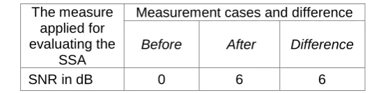
[image:12.595.159.428.402.469.2]

Results are given in Table 1 for comparison. A notable improvement for an average of about 6 dB has been achieved. This indicates a significant percentage in terms of signal energy. The result shown in the table is a reported average of a number of cases.

TABLE I. SNR MEASURE APPLIED FOR EVALUATING THE SSA FOR WIND NOISE REDUCTION The measure

applied for evaluating the

SSA

Measurement cases and difference

Before After Difference

SNR in dB 0 6 6

7

CONCLUSION AND DISCUSSION

This paper was set out as the first attempt to explore the SSA in microphone wind noise reduction in the context of outdoor sound acquisition for soundscapes and environmental sound monitoring. The plausible findings from the investigation suggest that microphone wind noise and wanted sound such as bird chirps are separatable by the SSA method, evidenced by a 6 dB reduction observed after the SSA de-noising as outlined in this paper.

The SSA is a model free and non-parametric method. The only parameter that can be adjusted is the window length. Nevertheless, the window length is known to have significant impact on the performance and effectiveness of the algorithm for specific application. The current results were obtained by a simplistic optimisation method. With systematic investigation and optimisation, the separability might be further improved.

Grouping is another key aspect to consider. The grouping technique reported in this paper is rather simplistic based on the Eigen-triple for separating the decomposed components after grouping similar components together. Even so, notable wind noise reduction was achieved. With more advanced grouping techniques such as w-correlation approach, the results might be further improved.

Vol. 39. Pt. 1. 2017

8

REFERENCES

1. Luzzi S, Natale R, Mariconte R. Acoustics for smart cities. AIA-DAGA Proc. 2013.

2. Slabbekoorn H. Songs of the city: noise-dependent spectral plasticity in the acoustic phenotype of urban birds. Anim Behav. 2013.

3. Schmidt MN, Larsen J, Hsiao F-T. Wind Noise Reduction using Non-Negative Sparse Coding. Mach Learn Signal Process 2007 IEEE Work. 2007:431-436. doi:10.1109/MLSP.2007.4414345.

4. Ma L, Milner B, Smith D. Acoustic environment classification. ACM Trans Speech Lang Process. 2006;3(2):1-22. doi:10.1145/1149290.1149292.

5. Chu S, Narayanan S, Kuo C. Environmental sound recognition using MP-based features.

Acoust Speech Signal …. 2008.

6. Nemer E, Leblanc W. Single-microphone wind noise reduction by adaptive postfiltering.

IEEE Work Appl Signal Process to Audio Acoust. 2009:177-180. doi:10.1109/ASPAA.2009.5346518.

7. King B, Atlas L. Coherent modulation comb filtering for enhancing speech in wind noise.

Proc Int Work Acoust Echo …. 2008.

8. Fukuda K. Noise reduction approach for decision tree construction: A case study of knowledge discovery on climate and air pollution. Comput Intell Data Mining, 2007. 2007. 9. Hassani H, Soofi A, Zhigljavsky A. Predicting daily exchange rate with singular spectrum

analysis. Anal Real World Appl. 2010.

10. Hassani H. A brief introduction to singular spectrum analysis. Optim Decis Stat data Anal [. 2010.

11. Hassani H, Heravi S, Zhigljavsky A. Forecasting European industrial production with singular spectrum analysis. Int J Forecast. 2009.

12. Hassani H, Dionisio A, Ghodsi M. The effect of noise reduction in measuring the linear and nonlinear dependency of financial markets. Nonlinear Anal Real World. 2010.

13. Ghodsi M, Hassani H, Sanei S, Hicks Y. The use of noise information for detection of temporomandibular disorder. Biomed Signal Process. 2009.

14. Hassani H, Zokaei M, Rosen D von, Amiri S. Does noise reduction matter for curve fitting in growth curve models? Comput methods. 2009.

15. Alonso F, Castillo J Del, Pintado P. Application of singular spectrum analysis to the smoothing of raw kinematic signals. J Biomech. 2005.

16. Elsner J, Tsonis A. Singular Spectrum Analysis: A New Tool in Time Series Analysis.; 2013. 17. Claessen D, Groth D. A beginner’s guide to SSA. CERES-ERTI, Ec Norm Super. 2002. 18. Alexandrov T. A Method of Trend Extraction Using Singular Spectrum Analysis.

2009;7(1):1-22.

19. Ghil M, Allen MR, Dettinger MD, et al. Advanced spectral methods for climatic time series.

Rev Geophys. 2002;40(1):1003. doi:10.1029/2000RG000092.

20. Patterson K, Hassani H, Heravi S. Multivariate singular spectrum analysis for forecasting revisions to real-time data. J Appl. 2011.