One dimensional vs two dimensional based features: Plant identification approach

One­dimensional vs. two­dimensional 

based features: Plant identification 

approach

Tharwat, A, Gaber, T and Hassanien, AE

http://dx.doi.org/10.1016/j.jal.2016.11.021

Title

One­dimensional vs. two­dimensional based features: Plant identification 

approach

Authors

Tharwat, A, Gaber, T and Hassanien, AE

Type

Article

URL

This version is available at: http://usir.salford.ac.uk/id/eprint/52075/

Published Date

2017

USIR is a digital collection of the research output of the University of Salford. Where copyright 

permits, full text material held in the repository is made freely available online and can be read, 

downloaded and copied for non­commercial private study or research purposes. Please check the 

manuscript for any further copyright restrictions.

One-Dimensional vs. Two-Dimensional based Features:

Plant Identication Approach

Alaa Tharwata,b_{, Tarek Gaber}b,c,1,∗_{, Aboul Ella Hassanien}b,d

a_{Faculty of Engineering, Suez Canal University, Egypt}

b_{Scientic Research Group in Egypt (SRGE), http://www.egyptscience.net} c_{Faculty of Computers and Informatics, Suez Canal University, Ismailia, Egypt}

d_{Faculty of Computers and Information, Cairo University, Egypt}

Abstract

The number of endangered species has been increased due to shifts in the

agri-1

cultural production, climate change, and poor urban planning. This lead to

2

investigating new methods to address the problem of plant species

identi-3

cation/classication. In this paper, a plant identication approach using 2D

4

digital leaves images was proposed. The approach used two features

extrac-5

tion methods based on one-dimensional (1D) and two-dimensional (2D) and the

6

Bagging classier. For the 1D-based methods, Principal Component Analysis

7

(PCA), Direct Linear Discriminant Analysis (DLDA), and PCA+LDA

tech-8

niques were applied, while 2DPCA and 2DLDA algorithms were used for the

9

2D-based method. To classify the extracted features in both methods, the

Bag-10

ging classier, with the decision tree as a weak learner was used. The ve

11

variants, i.e. PCA, PCA+LDA, DLDA, 2DPCA, and 2DLDA, of the approach

12

were tested using the Flavia public dataset which consists of 1907 colored leaves

13

images. The accuracy of these variants was evaluated and the results showed

14

that the 2DPCA and 2DLDA methods were much better than using the PCA,

15

PCA+LDA, and DLDA. Furthermore, it was found that the 2DLDA method

16

was the best one and the increase of the weak learners of the Bagging classier

17

yielded a better classication accuracy. Also, a comparison with the most

re-18

lated work showed that our approach achieved better accuracy under the same

19

dataset and same experimental setup.

20

Keywords: Plant Identication, Principal Component Analysis, Linear

∗_{Corresponding author}

Email addresses: [email protected] (Alaa Tharwat ), [email protected] (Tarek Gaber ), [email protected] ( Aboul Ella Hassanien)

Discriminant Analysis (LDA), Bagging classier, weak learners, 2DLDA, 2DPCA, Direct-LDA, Leaf Image, Leaves Images, Small Sample Size (SSS), PCA+LDA

1. Introduction

21

Plants are a vital element of the Earth's ecology system. They maintain a

22

healthy breathable atmosphere. Almost the entire oxygen, needed for humans

23

and other animals breathe, are produced by plants, thus without plants, there

24

is no life on the earth (Gaber et al., 2015; Chaki et al., 2016). In addition,

25

plants can be used as an alternative energy source, e.g., bio-fuel (Chaki and

26

Parekh, 2012). There are various species of plants which are subject to the

27

danger of extinction. Saving endangered species of these plants from becoming

28

extinct and protecting their wild places is important for our health and the

29

future of our children. The impact of biodiversity loss may lead to fewer new

30

medicines, greater vulnerability to natural disasters and greater eects from

31

global warming. Therefore, there is a need for protecting plants and classifying

32

them into dierent species. For this purpose, plant identication techniques

33

have become a hot area of research.

34

Traditional plant identication can be achieved by a manual matching of

35

the plant's characteristics including leaves, fruits, owers, and stem, against

36

an atlas. Such identication requires extensive knowledge and it makes use of

37

complex terminology in a way that even a professional botanist needs to spend

38

much time in a eld to achieve plant identication. The plant identication

39

could be automatically achieved through using the plants' features that are

ex-40

tracted from their images and then these features can be classied using various

41

classier techniques such as, Neuro-Fuzzy Classier (Chaki et al., 2016),

Sup-42

port Vector Machine (SVM) (Arun Priya et al., 2012a), etc. Since some plants'

43

owers and fruits are seasonal and their colors are changed according to the

44

season, the leaves are more suitable to identify plants than owers and fruits.

45

Hence, the majority of the existing computer-based plant identication has used

the leaves of plants (Chaki and Parekh, 2012; Chaki et al., 2015, 2016). The

47

automatic plant identication based on information technology is a very vital

48

task for dierent parties: agriculture, pharmacological, forestry science.

Auto-49

matic plant identication process will achieve fast, cheap, and accurate systems,

50

which provide a great help to medicine, industry, and foodstu production, as

51

well as to biologists, chemists, and environmentalists.

52

This paper describes an approach addressing the plant identication

prob-53

lem by using features that are extracted from digital images of plant leaves as it

54

is a low-cost and convenient way to get leaf images dataset. The approach used

55

two features extraction techniques (one-dimensional (1D) and two-dimensional

56

(2D) based) with the Bagging classier. For the 1D-based techniques, PCA,

57

PCA+LDA, and Direct-LDA techniques were applied, while 2DPCA and 2DLDA

58

algorithms were used for the 2D-based method. To classify the extracted

fea-59

tures in both methods, the Bagging classier, with the decision tree as a weak

60

learner was used.

61

The rest of the paper is organized as follows; Section (2) summarizes the

62

related work of the plant identication based on machine learning. Section (3)

63

highlights the feature extraction methods and the classier used in the design

64

of the proposed approach which is presented in Section (4). The experimental

65

results are reported in Section (5) while the results' discussion and the conclusion

66

are presented in Section (6) and Section (7), respectively.

67

2. Related Works

68

There are a number of plant identication approaches that used digital

im-69

ages (Valliammal and Geethalakshmi, 2011; Arora et al., 2012; Arun Priya et al.,

70

2012b; Satti et al., 2013). Satti et al. classied plant leaves based on 2D

im-71

ages. They used Flavia image dataset and applied many preprocessing steps on

72

the leaf images (Satti et al., 2013). Their approach achieved accuracy 85.9%

73

and 93.3% using k-Nearest Neighbour (k-NN) and Articial Neural Networks

74

(ANN) classiers, respectively. Arora et al. applied the Speed Up Robust

tures (SURF) to extract the features from leaf images and then used the Random

76

Forest (RF) classier and tested their approach using Plant Leaves II dataset

77

(Arora et al., 2012). In another research, Caglayan et al. utilized color and

78

shape features to classify 32 dierent kinds of plants. They used SVM, k-NN,

79

RF, and Naive Bayes (NB) classiers and the RF classier achieved the best

80

accuracy (96%) (Caglayan et al., 2013). Arun et al. transformed the leaf images

81

into grayscale and applied boundary enhancement operations (Arun Priya et al.,

82

2012b). They then used the PCA to extract features and then used SVM and

83

k-NN for classication. They used Flavia dataset and achieved the accuracy of

84

78% to 81.3% using k-NN classier.

85

Valliamma et al. proposed identication approach for ower images dataset

86

(Valliammal and Geethalakshmi, 2011). They applied Preferential Image

Seg-87

mentation (PIS) and other enhancement operations to the images. They then

88

used the image thresholding to obtain some features and then used the

prob-89

abilistic curve for classication. They used a dataset of 500 owers images.

90

In another research, Uluturk and Uger converted the plant leaf images into

91

grayscale, the region of interest was segmented and the features were extracted

92

(Uluturk and Ugur, 2012). Probabilistic Neural Networks (PNN) classier was

93

then used of Flavia dataset and the classication rate was 92.5%.

94

Recently, Chaki et al., proposed a plant recognition approach using both of

95

texture and shape features (Chaki et al., 2015). The texture features were

ex-96

tracted by Gray Level Co-occurrence Matrix (GLCM) and Gabor lter while the

97

shape features were extracted using the curvelet transform coecients and the

98

invariant moments. This approach was tested using two neural-based classiers:

99

a feed-forward back-propagation Multi-Layered Perceptron (MLP) and a

Neuro-100

Fuzzy Classier (NFC) to classify 31 plant species of leaves images. In another

101

study, (Chaki et al., 2016) proposed another approach based on ridge lter and

102

curvelet transform with a Neuro-Fuzzy classier. The classication accuracy of

103

almost all classes (plant species) was 100%. However, it needs preprocessing

104

step which imposes more CPU time.

3. Preliminaries

106

In this section, the background of the PCA and LDA methods are introduced.

107

Moreover, the details of how to use both methods in vector or matrix form are

108

explained below.

109

3.1. Feature Extraction Method

110

The aim of the feature extraction step is to transform the objects'

proper-111

ties into numeric values. There are many types of features for an image such as

112

shape, texture, and color features. The shape features are used to describe the

113

shape of the image or the Region of Interest (ROI) while the texture features

114

describe the texture analysis of the image. The texture features methods are

115

generally classied into two methods: sparse method and dense method. In

116

the sparse method, the interest points are rst detected and then a local patch

117

around these points is constructed, and nally, invariant features are extracted.

118

Scale Invariant Feature Transformation (SIFT) is one of the most common

al-119

gorithms in the sparse descriptor method (Lowe, 1999; Tharwat et al., 2015). In

120

the dense method, the local features are extracted from each pixel over the input

121

image. Local Binary Patterns (LBP) is one of the most common algorithms in

122

dense method (Ojala et al., 2002; Tharwat et al., 2014b). The color features are

123

widely used in image retrieval due to its robustness against image size variation

124

and orientation (Salvador et al., 2004). The feature extraction techniques used

125

in the proposed approach are highlighted below.

126

3.1.1. An Overview of PCA

127

(PCA) is one of the classical feature extraction techniques that is widely

128

used in the areas of pattern recognition and computer vision since Turk and

129

Pentland (Turk and Pentland, 1991) used it for face recognition in 1991. From

130

that time, PCA has been widely used in face recognition and many other pattern

131

recognition applications such as dimensionality reduction (Moore, 1981), face

132

recognition (Turk and Pentland, 1991; Yang et al., 2004), and ear recognition

133

(Tharwat et al., 2012).

The PCA is an unsupervised method that is used to search for a new space

135

(PCA space or eigen space), WP CA, which reduces the d-dimensional feature

136

vectors tok-dimensional feature vectors (wherek < d).

137

Given I = {I1, I2, . . . , IM}, whereIi ∈ Rd is the ith pattern or sample,d

138

is the dimension or the number of features of Ii, and M is the total number

139

of samples. PCA searches for the PCA space (WP CA) which represents the

140

direction of the maximum variance of the given data. The PCA space consists

141

ofkorthonormal and uncorrelated Principal Components (PCs). The rst step

142

of the PCA method is to calculate the covariance matrixΣas follows:

143

Σ = 1

M −1D×D

T_{, (1)}

D={d1, d2, . . . , dM}= M

X

i=1

Ii−µ (2)

whereµ= _M1 PM

i=1Iiis the mean of all samples. The eigenvalues ({λ1, λ2, . . . , λd})

144

and eigenvectors ({v1, v2, . . . , vd}) of Σ are then calculated. The eigenvector

145

with the highest eigenvalue represents the rst principal component and it has

146

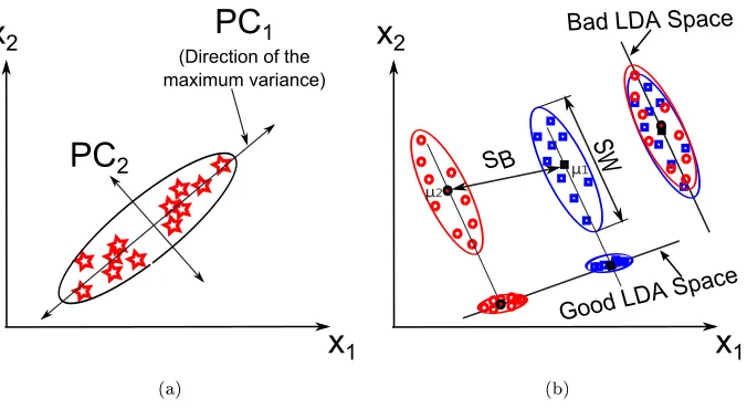
the maximum variance as shown in Figure 1a (Turk and Pentland, 1991; Strang,

147

2003). As shown in the gure, the rst principal component (PC1) points to the

148

maximum variance. Algorithm (1) summarizes the steps of the PCA technique.

149

3.1.2. An Overview of LDA

150

LDA is also a well-known algorithm for feature extraction and

dimensional-151

ity reduction. LDA is widely used in dierent applications such as biometrics

152

(Marcialis and Roli, 2002; Tharwat et al., 2014a), bioinformatics (Wu et al.,

153

2009), and chemoinformatics (Mitchell, 2014). LDA is a supervised

dimension-154

ality reduction and feature extraction method (Galdámez et al., 2015). It nds

155

the projection space that maximizes the ratio of the between-class variance,

156

SB, to the within-class variance, SW, and hence guaranteeing maximum class

157

separability as shown in Figure 1b (Welling, 2005). From the gure, there are

158

two sub-spaces that can be selected to represent the LDA space. As shown, in

x

x

PC

(Direction of the maximum variance)

PC

(a)

x

x

SB

μ2

S

W

Good LDA S

pace

Bad LDA Space

(b)

Figure 1: A visualization of the PCA and LDA techniques; (a) PCA, (b) LDA.

Algorithm 1 : PCA

1: Given a feature matrix which consists of all training samples, each sample is represented by a single column as follows,I= [I1, I2, . . . , IM] , whereM

represents the total number of samples,Ii represents a training sample.

2: Compute the mean of all classes (total mean)µ= _M1 PM

i=1Ii. 3: Subtract the mean from all training samples as follows,Di=Ii−µ.

4: Compute covariance matrixCov=_M1₋₁PM

i=1Di∗DiT.

5: Compute eigenvectorsV and eigenvalues λof the covariance matrix.

6: Sort eigenvectors according to their corresponding eigenvalues.

7: Select k eigenvectors that have the largest eigenvalues WP CA =

{v1, v2, . . . , vk}. The selected eigenvectors represent the projection space

of PCA (WP CA).

the bad LDA space, the two classes cannot be discriminated because the SB

160

between the two classes decreased. On the other hand, in the good LDA space,

161

SW is decreased whileSB is increased and hence the two classes are perfectly

162

discriminated.

163

Assume the training samples belong to C classes. The aim of the LDA

method is to search for the subspace,WLDA, which maximizesSBand minimizes

165

SW as follows:

166

J(w) = W

T

LDASBWLDA

WT

LDASWWLDA

, (3)

SB = C

X

i=1

ni

M(µi−µ)(µi−µ)

T_{, (4)}

S_Wi = 1

ni ni

X

j=1

(I_ji−µi)(Iji−µi)T, (5)

SW = C

X

i=1

ni

MS

i

W (6)

where ni is the number of samples of classi, µi = _n1

i

Pni

j=1Iji is the mean of

167

classi,µ=_C1 PC

i=1µi= _M1 P M j=1I

i

j represents the global mean or the mean of

168

all samples,I_ji is the jth sample in theith class,M =PC

i=1ni, andSWi is the

169

within-class matrix of theith class. Algorithm (2) summarizes the steps of the

170

LDA technique.

171

In practice, SW is always singular, this is the so-called singularity, Small

172

Sample Size (SSS), or under-sampled problem. This problem is common in LDA

173

technique and it results from high-dimensional pattern classication applications

174

or a small number of training samples available for each class compared with the

175

dimensionality of the sample space (Lu et al., 2005; Ye and Xiong, 2006). The

176

SSS problem occurs when theSW is singular2. The upper bound of the rank3

177

ofSW isM−C, while the dimension ofSW isd×d(Lu et al., 2005; Feng and

178

Wu, 2014). Thus, in most casesd >> M−Cwhich leads to SSS problem. For

179

example, in face recognition applications, the size of the face image may reach

180

2_{A matrix is singular if it is square, does not have a matrix inverse, and/or its determinant}

is zero; hence not all columns and rows are independent (Strang, 2003).

3_{The rank of the matrix represents the number of linearly independent rows or columns}

to 100×100 = 10000pixels, which represent high-dimensional features and it

181

leads to a singularity problem.

182

There are two common solutions to SSS problem. The rst solution is to

183

use a non-singular intermediate, e.g. PCA space, to reduce the dimension of

184

the original data to be equal to the rank ofSW, hence SW becomes full-rank

185

andSW can be inverted. The second solution is to remove the null-space ofSB

186

which contains no useful information for recognition by diagonalizing SB and

187

then diagonalizingSW. These two solutions were used in this paper.

188

Algorithm 2 : Linear Discriminant Analysis (LDA)

1: Given a set ofM samples[Ii]Mi=1, each of which is represented as a column as follows,I= [I1, I2, . . . , IM]and each sample is represented bydfeatures.

2: Compute the mean of each class,µi, and the total mean of all samples,µ.

3: Compute within-class scatter matrix, SW, as in Equations (5 and 6) and

the between-class scatter matrixSB as in Equation (4).

4: Calculate the eigenvalues (λ) and eigenvectors (V) ofS_W−1SB as follows:

SBV =SWV λ (7)

5: Sort the eigenvectors in descending order according to their corresponding eigenvalues, then use the rst,k, eigenvectors as a lower dimensional space

(WLDA).

3.1.3. One-Dimensional Feature Extraction Technique:

189

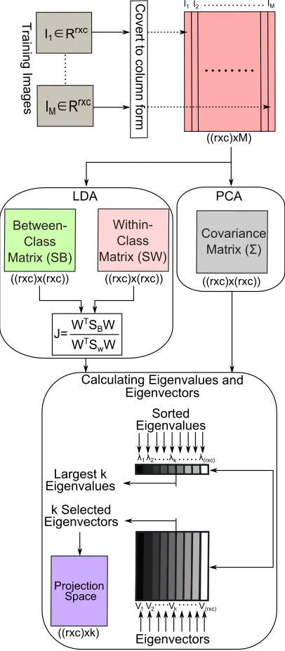
The classical PCA (i.e. 1DPCA) and LDA (i.e. 1DLDA) use one-dimensional/vector

190

form to calculate projection spaces as shown in Figure 2. In both methods, a

191

two-dimensional image (Ii(r×c), ∀i= 1,2, . . . , M) is rst converted into one

192

feature vector (column or row), where r and c represent the number of rows

193

and columns of the image, respectively. All the feature vectors are then

con-194

catenated to form a feature matrix (I ={I1, I2, . . . , IM}), whereM refers to

195

the total number of images. The PCA and LDA spaces,WP CAand WLDA, of

196

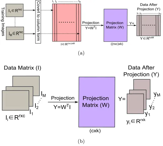
this matrix (I) can be calculated. The features are then extracted by

ing the feature matrix on the calculated spaces as follow,Y =WTI, whereW

198

represents the lower dimensional space (i.e. PCA or LDA) (see Figure 3a).

199

I1I2

wwrxcJxMJ

IM

Train

ingEImage

s

I1∈Rrxc

wwrxcJxwrxcJJ

PCA

CovarianceE MatrixEwΣJ

I

∈

R

CovertEtoEcolum

nEform

λ1λ2 λwrxcJ

V1V2 VwrxcJ

Sorted Eigenvalues

Eigenvectors kESelected

Eigenvectors

Vk λk

LargestEkE Eigenvalues

Projection ESpace

wwrxcJxkJ

CalculatingEEigenvaluesEandE Eigenvectors

LDA

wwrxcJxwrxcJJ wwrxcJxwrxcJJ

WT_S

BWEE

WT_S

wW

J=

Within-ClassE MatrixEwSWJ

Between-ClassE MatrixEwSBJ

Vector representation may lead to a high-dimensional data. Hence, it is

dif-200

cult to calculate the covariance matrix in PCA due to its large size. Moreover,

201

the high-dimensional data leads to SSS problem in LDA. These two problems

202

can be solved using the two-dimensional methods, i.e. 2DPCA and 2DLDA.

203

Projection

Y∈RkxM DataCAfterC ProjectionC(Y)

Y=WT_I

I∈R(rxc)xM

Y=

((rxc)xk) ProjectionC MatrixC(W)

y1y2 yM I1I2 IM

Train

ingCImage

s

I1∈Rrxc

IM∈Rrxc

CovertCtoCcolum

nCform

(a)

Projection

yi∈Rrxk Data After Projection (Y)

Y=WT_I

Data Matrix (I)

Y=

(cxk) Projection Matrix (W)

Ii∈Rrxc

I1

I2

IM

y1 y2

yM

(b)

Figure 3: A visualization of the projection of one-dimensional and two-dimensional methods; (a) one-dimensional method, (b) two-dimensional method.

3.1.4. Two-Dimensional Feature Extraction Techniques

204

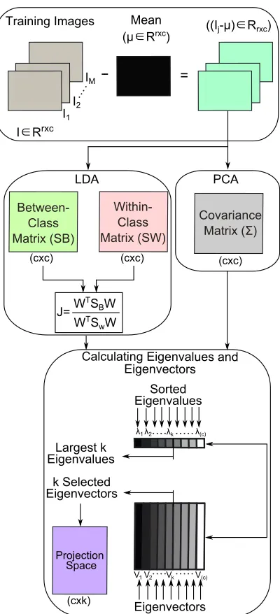
The spaces of the PCA and LDA techniques can be calculated in

two-205

dimensional/matrix form, i.e. 2DPCA and 2DLDA, as shown in Figure 4.

206

Hence, there is no need for the step of converting each image into one

vec-207

tor prior to feature extraction step which saves more computational time. As in

208

one-dimensional technique, the PCA and LDA spaces, WP CA and WLDA, are

209

calculated and the features are then extracted by projecting the feature matrix

210

on the calculated spaces as follows,Y =WT_{I(see Figure 3b).}

3.1.4.1. Two Dimensional PCA (2DPCA). The aim of the 2DPCA method is

212

to nd the PCA space,WP CA, to project the two-dimensional image (Ii∈ Rr×c)

213

as follows,Yi =WP CAT Ii, whereYi is the projected feature vector of the image

214

Ii. First, the M two-dimensional images are used to calculate the covariance

215

matrix (Σ∈ Rc×c_{) as in Equation (8). The eigenvalues and eigenvectors ofΣ}

216

are then calculated andkoptimal eigenvectors, i.e. projection axes, are selected.

217

In other words, the 2DPCA method then searches for the PCA spaceWP CA=

218

{v1, v2, . . . , vk} which maximizes the variance as in classical PCA, wherevi is

219

theith _{principal component and k is the number of selected eigenvectors that}

220

represent the PCA space. This projection space is used for feature extraction of

221

the image as follows,Yi =WP CAT Ii, where Yi ∈ Rr×k represents the projected

222

feature vectors, i.e. feature matrix or feature image, of the imageIi(Yang et al.,

223

2004).

224

Σ = 1

M −1

M

X

j=1

(Ij−µ)T(Ij−µ) (8)

whereµis the mean of all training images,M is the number of training images,

225

andIj represents thejthtraining image.

226

3.1.4.2. Two Dimensional LDA (2DLDA). The aim of the 2DLDA method is

227

to nd the LDA space, WLDA, to extract the features by projecting the

two-228

dimensional image on the LDA space usingYi=WLDAT Ii. AssumeIirepresents

229

one image and M two-dimensional images are used to calculate within-class

230

matrix (SW) and between-class variance (SB). The eigenvalues and eigenvectors

231

ofS−_W1SB are then calculated andk optimal eigenvectors are selected to form

232

the LDA space, i.e. Fisher projection matrix using WLDA = {v1, v2, . . . , vk}

233

which maximizes the ratio betweenSB andSW as in classical LDA, whereviis

234

theith_eigenvector.

235

3.2. The Bagging Classier

236

The Bagging classier is one of the ensemble classiers creating its ensemble

237

by training dierent classiers or weak learners on a random distribution of

TrainingkImages

ــ

Meank Bμ∈Rrxc_w

=

BBIj-μw∈Rrxcw

I∈Rrxc

λ1λ2 λBcw

V1V2 VBcw

Sorted Eigenvalues

Eigenvectors kkSelected

Eigenvectors

Vk λk

Largestkkk Eigenvalues

Projection kSpace

Bcxkw

CalculatingkEigenvalueskandk Eigenvectors I1

I2

IM

Bcxcw

PCA

Covariancek MatrixkBΣw

LDA

WT_S BWkk

WT_S wW

J=

Within-Classk MatrixkBSWw

Between-Classk MatrixkBSBw

Bcxcw Bcxcw

Figure 4: Visualized steps to calculate a projection space of two-dimensional PCA and LDA (2DPCA and 2DLDA) methods.

a training dataset. A weak learner is a simple, fast, and easy to implement

239

classier such as single level decision tree or simple neural networks (Kuncheva,

240

2014).

Generally, as given in Algorithm (3), a Bagging classier consists of two

242

phases: training and testing. In the training phase, for each iteration, t, a

243

number of training samples are selected randomly (Si), and these samples are

244

used to train one weak learner (Ct) as shown in Figure 5. In the testing phase, all

245

the weak learners are used to classify an unknown sample (Itest). The outputs

246

of all weak learners are combined using majority voting method to determine

247

the nal decision (Kuncheva, 2014).

248

Algorithm 3 Bagging Classier Algorithm

1: Given a training setI= (I1, y1), . . . ,(IM, yM), whereyirepresents the label

of samplesIi ∈IandM denotes the total number of samples in the training

set.

2: while (t < T) do

3: Select a sampleStfromI.

4: UseStto train the current weak learnerCt.

5: end while

6: Given new test patternItest.

7: ClassifyItest using all weak learners.

8: Combine the outputs of all weak learners to determine the nal prediction.

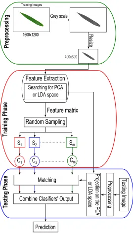
4. Proposed Approaches

249

The proposed plant identication approach consists of two phases. In the

250

rst phase, two main feature extraction methods (1D-based and 2D-based) were

251

used. In the 1D-based feature extraction method, 1DPCA, Direct LDA (DLDA),

252

and (PCA+LDA) techniques were used while in the 2D-based method, 2DPCA

253

and 2DLDA were applied for the feature extraction step. For the identication,

254

in both techniques, the Bagging classier was used to identify the type of the

255

unknown leave image as shown in Figure 5. As shown in Figure 5, the proposed

256

model has two main phases: training and testing phases.

4.1. Training Phase

258

In the training phase, M images (IM

i=1) were used to train the proposed

259

model. In the 1D-based method, each image was rst transformed into one

260

vector and then all training images' vectors were combined into a matrix,I =

261

[I1, I2, . . . , IM](see Figure 2). In the 2D-based method, the training image was

262

not changed but represented as 2D matrix as seen in Figure 4. The PCA or LDA

263

spaces,W, of I were then constructed. The features were then extracted from

264

all training images by projecting the images on the space. These features were

265

used to train the Bagging model. The steps of the training phase are explained

266

in detail in Algorithm (4).

267

Algorithm 4 : Training Phase 1: Read the training images.

2: if (1D-based method) then

3: Convert all imagesIi(r×c), i= 1, . . . , M into vectorsIi((r×c)×1).

4: Combine all feature vectors into a matrix (I= [I1, I2, . . . , IM]).

5: else

6: Deals with images in 2D form (i.e. matrix representation).

7: Combine all feature vectors into a matrix (I= [I1, I2, . . . , IM]).

8: end if

9: Compute the projection space (W).

10: Project I on the projection surface (W) to obtain the features as follows, Y =WT_I.

11: Train the Bagging classier using the extracted features,Y.

4.2. Testing Phase

268

In the testing phase, an unknown leave image (Itest) was tested for its plant

269

identication. To do so, rstly the leave features were extracted by projecting

270

it on the projection space, W, that was computed in the training phase, i.e.

271

Ytest = WTItest. The computed vector Ytest was classied using the Bagging

S

CombineEClasifiersyEOutput

TestingEImag

e

RandomESampling

S

S

S

C

C

C

Training Phas

e

Matching

Prediction

Testing

Phase

TrainingEImages

FeatureEExtraction

SearchingEforEPCAE

orELDAEspace

FeatureEmatrix

Proj

ectionEonEtheEPC

AE

orELDA

Espace

GreyEscale

Resize

Preproces

sing

Prep

rocessin

gE

1600x1200

400x300

Figure 5: Plant identication system using leaves' images

classier's model that has been also built in the training phase. Detailed steps

273

of this phase are given in Algorithm (5)

Algorithm 5 : Testing Phase

1: Read an unknown leave image (Itest).

2: if (1D-based method)) then

3: Convert this imageItest(r×c)into a vector form,Itest´ ((r×c)×1).

4: else

5: Deals with the image in 2D form (i.e. matrix representation).

6: end if

7: Project the unknown 2D image on the projection space to getytest.

8: Match betweenytest withY using the Bagging model that built during the

training phase to nd the class label of the unknown image.

5. Experimental Results

275

To evaluate our proposed approach, the Flavia public dataset was used.

276

This dataset consists of 1907 colored leaves images with size (1600×1200)

277

and collected from 33 dierent species. The selected images are in dierent

278

orientations, illumination, and quality. In this paper, all colored images were

279

converted into grey scale images as shown in Figure 5. Next, all images were

280

resized to be 400×300 to reduce the computational time. Figure 6 shows

281

dierent samples from the dataset.

282

Four scenarios were designed to evaluate the performance and accuracy of the

283

proposed model (using 1DPCA, PCA+LDA, DLDA, 2DPCA, and 2DLDA). In

284

these scenarios, the Bagging classier ensemble, with dierent numbers of weak

285

learners was used to match the unknown image with the trained images. Due

286

to the high dimensionality of the data, 1DLDA was not suitable for the feature

287

extraction. The reason of this high-dimensionality of the one-dimensional form

288

of the image wasd= 400×300 = 120000and henced >> M−Cwhich leads to

289

SSS problem, whereM is the total number of samples andC is the number of

290

classes. To avoid this problem, PCA+LDA and Direct LDA (DLDA) methods

291

were used for the feature extraction in the one-dimensional method.

292

In the rst scenario, the accuracy of the two methods (1D-based and

Figure 6: Sample of dierent leaves' images (one sample from each class or plant).

based) was investigated through testing dierent percentages of training images

294

of each plant type, i.e. class. The training images were selected randomly from

295

the database while the remaining images, were used during the testing phase.

In this scenario, the size of Bagging classier was ve. The accuracy and CPU

297

time of this scenario are shown in Figure 7.

298

10 20 30 40 50 60 70 80 90

45 50 55 60 65 70 75 80 85 90 95

Number of Training Images

Accuracy (%) 1DPCA

PCA+LDA DLDA 2DPCA 2DLDA

(a)

10 20 30 40 50 60 70 80 90

0 0.01 0.02 0.03 0.04 0.05 0.06 0.07 0.08 0.09 0.1

Percentage of Training Images (%)

CPU Time (sec)

1DPCA PCA+LDA DLDA 2DPCA 2DLDA

(b)

Figure 7: Accuracy and CPU time of the proposed model using 1DPCA, PCA+LDA, DLDA, 2DPCA, and 2DLDA with dierent percentages of the training images and ve weak learners of the Bagging classier; (a) Accuracy, (b) CPU time.

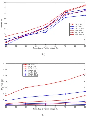
The second scenario was designed based on the results of the rst one in

10 20 30 40 50 60 70 80 90 60

65 70 75 80 85 90 95 100

Percentage of Training Images (%)

Accuracy (%)

2DLD−5C 2DLD−51C 2DLD−201C 2DPCA−5C 2DPCA−51C 2DPCA−201C

(a)

10 20 30 40 50 60 70 80 90

0 0.1 0.2 0.3 0.4 0.5 0.6 0.7

Percentage of Training Images (%)

CPU Time (sec)

2DLD−5C 2DLD−51C 2DLD−201C 2DPCA−5C 2DPCA−51C 2DPCA−201C

(b)

Figure 8: Accuracy and CPU time of the 2D-based method with dierent number of training images and weak learners of the Bagging classier.

which the 2D-based methods gave better results than that of the 1D-based one.

300

Thus, the aim of this scenario was to further understand the eect of changing

301

the number of training images and to evaluate the accuracy and the performance

302

stability over the standardize data. In this scenario, the 2DPCA and 2DLDA

303

were used to extract the images' features. The Bagging classier was then used

304

in many experiments at dierent values of its weak learners (i.e. 5, 51, and

0 50 100 150 200 250 300 350 400 450 86

88 90 92 94 96 98 100

Ensemble Size

Accuracy (%)

2DLDA−Test 2DLDA−Training 2DPCA−Test 2DPCA−Training

Figure 9: A comparison between the training and testing accuracy of 2DLDA and 2DPCA method using dierent ensemble sizes.

201). In addition, the percentage of training images was ranged from 10% to

306

90%. The results obtained from this scenario are shown in Figure 8. Moreover,

307

a comparison between the training and testing accuracy of the Bagging model

308

is shown in Figure 9.

309

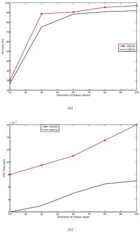
The third scenario was conducted to investigate the relationship between the

310

accuracy and the dimension of the feature vectors of the 2DPCA and 2DLDA

311

methods. In other words, the accuracy of the 2DPCA and 2DLDA was tested

312

against dierent numbers of eigenvectors constructing the projection space. In

313

this experiment, series of dierent dimensions were used. Moreover, 90% of the

314

images from each class were used to train the model, while the other images

315

were used to test the model. In addition, there were 51 weak learners in the

316

Bagging classier. Figure 10 shows the results of this experiment.

317

The fourth and last scenario was conducted to compare the accuracy of the

318

2DLDA method when dierent classiers (Bagging,k-NN, and MLP) were used.

319

In all experiments of this scenario, 51 weak learners were used in the Bagging

20 30 40 50 60 70 80 90 100 10

20 30 40 50 60 70 80 90 100

Dimension of Feature Vectors

Accuracy (%)

2DLDA 2DPCA

(a)

20 30 40 50 60 70 80 90 100

2 4 6 8 10 12 14 16x 10

−3

Dimension of Feature Vector

CPU Time (sec)

2DLDA 2DPCA

(b)

Table 1: Accuracy rate of the proposed model using Bagging,k-NN, and MLP classiers.

Class Bagging k-NN MLP Class Bagging k-NN MLP Class Bagging k-NN MLP

1 98 94 98 12 100 94 92 23 98 94 96

2 100 90 98 13 100 86 94 24 100 90 96

3 97 90 95 14 96 86 92 25 100 92 94

4 100 94 96 15 98 92 92 26 98 94 94

5 96 96 96 16 92 90 92 27 98 94 96

6 98 90 92 17 96 92 92 28 98 90 96

7 100 92 88 18 96 82 88 29 100 92 97

8 96 85 90 19 98 94 96 30 98 90 94

9 94 88 86 20 96 92 96 31 92 87 92

10 98 92 94 21 92 87 90 32 98 86 92

11 98 84 92 22 86 81 82 33 100 96 96

classier, ve nearest neighbours (k = 5) in the k-NN classier, and 30 and

321

33 nodes for the hidden and output layers, respectively, in the MLP classier.

322

Moreover, 90% of the images from each class were used to train the model, while

323

the other images were used to test the model. The accuracy of each class of this

324

experiment are summarized in Table 1

325

6. Discussion

326

From the results of the rst scenario, shown in Figure 7, the following

re-327

marks can be drawn. Firstly, in terms of accuracy issues, the accuracy of all ve

328

variants (i.e. 1DPCA, PCA+LDA, DLDA, 2DPCA, and 2DLDA) was improved

329

when the number of training images was increased. This can be explained, as

330

reported in (Brain et al., 1999), using more training images will decrease the

331

variance4 _{and hence decreases the overtting. Secondly, the accuracy of the}

332

2D-based methods (i.e. 2DPCA and 2DLDA) was better than that of the

1D-333

based methods (i.e. 1DPCA, PCA+LDA, and DLDA). Thirdly, the 2DLDA

334

method achieved the best accuracy and the 1DPCA-based one accomplished

335

the worst accuracy. Fourthly, DLDA method achieved accuracy better than

336

PCA+LDA method because PCA+LDA method loses more information than

337

DLDA as mentioned in Section 3.1.2.

338

In terms of the CPU performance, from Figure 7b, it can be noticed that

339

the 2DPCA is the most ecient algorithm among all other methods and the

340

DLDA is the worst one. This can be explained as the high dimensionality of the

341

one-dimensional data. Mathematical interpretation of this point shows that the

342

size of the image covariance matrix using 2DPCA (c×c) is much smaller than

343

in 1DPCA ((r×c)×(r×c)). As a result, less time is required to determine

344

the corresponding eigenvectors when the 2DPCA is used. For example, in our

345

case, the size of the image after resizing it was400×300. Hence, to calculate

346

the covariance matrix of 2DPCA, it is required to multiply two matrices of

347

(300×300). But, when using the 1DPCA, all training images are converted into

348

one vector (1×120000), and the covariance matrix is computed by multiplying

349

two matrices(M×120000)×(120000×M), whereM represents the total number

350

of training images. Thus, 2DPCA method takes CPU time much lower than

351

1DPCA method. Similarly, 2DLDA involves the eigen-decomposition of matrix

352

SW andSB which have dimensions much smaller than in 1DLDA method. This

353

reduction dramatically reduces the computational time and memory space of

354

2DLDA method (Ye et al., 2004). Moreover, in 1DLDA,SW is singular in most

355

cases because the dimension of the samples is greater than the number of samples

356

in each class. However, 2DLDA overcome this problem eciently because the

357

rank of any training image is equal tomin(r, c). Hence, the rank ofSW is less

358

than or equal to(M−C).min(r, c)(Li and Yuan, 2005). Thus, in 2DLDA,SW

359

is nonsingular when Equation (9) is true. In real practical problems, Equation

360

(9) is always satised. Thus,SW is always nonsingular, hence, SSS problem can

361

be solved using 2DLDA (Li and Yuan, 2005).

362

M ≥C+ c

min(r, c) (9) From Figure 8 the following remarks can be noticed. Firstly, the higher

363

number of iterations of Bagging classier used, the better classication accuracy

achieved. However, this was accomplished on the cost of taking more CPU time

365

(see Figure 8b). Secondly, the 2DLDA method achieved identication accuracy

366

better than that of the 2DPCA method, but this was also accomplished with

367

more CPU time. This is because of LDA searches in the space that extracts the

368

most discriminative features, while the PCA searches in the space that extracts

369

the data with the high variance. Thirdly, increasing the ensemble size led to the

370

complexity of the bagging model and hence took more CPU time and may lead to

371

the overtting problem. Figure 9 shows a comparison between the training and

372

testing accuracy. In this gure, the training accuracy of 2DLDA and 2DPCA

373

methods was increased till it reached to an extent at which it remained constant.

374

On the other hand, the testing accuracy was increased when the ensemble size

375

was increased till it reached to an extent after which it reduced again. As shown

376

in the gure, the best ensemble size was approximately 201.

377

From Figure 10a, two remarks can be noticed. First, the accuracy of the

378

2DPCA and 2DLDA methods is proportional with the number of eigenvectors.

379

Second, a major change (about 60%) in the accuracy achieved when the

percent-380

age of the eigenvectors was increased from 20% to 40%. But, a minor change

381

(about 5%) in the accuracy achieved when the percentage of the accuracy ranged

382

from 40% to 100 %. This means that the most discriminative feature are

con-383

centrated nearly in the rst half of the eigenvectors. In terms of CPU time and

384

from Figure 10b, it is clear the computational time of the 2DPCA and 2DLDA

385

methods increased when more eigenvectors were used to construct the PCA or

386

LDA space.

387

From Table 1, two remarks can be seen. First, the Bagging classier achieved

388

the best accuracy rate (97.15%), while MLP and k-NN classiers achieved

389

93.15% and 90.18%, respectively. The accuracy of the classes was ranged from

390

86% to 100% when Bagging classier was used.

391

To further evaluate our proposed approach (2DPCA and 2DLDA which gave

392

the best results), a comparison was conducted with some state-of-the-art

ap-393

proaches which used dierent feature extraction methods and classiers for the

394

same dataset. The results of this comparison are shown in Table 2. From this

Table 2: A comparison between our proposed plant identication method and some of state-of-the-art methods in terms of, classication accuracy, size of database images, feature extraction methods.

Author Feature Extraction Method

Classication Method

Database

Images Results

(Arun Priya et al., 2012b) Digital Morphological Features (DMFs) + PCA

k-NN

SVM

5 classes (331 images)

k-NN (78%)

SVM (94.5%)

(Caglayan et al., 2013) Color+Shape

k-NN

SVM NB RF

32 classes (1897 images)

k-NN (94.2%)

SVM (92.9%) NB (88.95%) RF (96.32%)

(Satti et al., 2013) Color+Shape k-NN ANN

33 classes (1907 images)

k-NN (85.9%) ANN (93.3%)

(Chaki et al., 2015) Texture+Shape NFC MLP

31 classes (930 images)

NFC (81.6%) MLP (87.1%)

(Chaki et al., 2016) Shape+Texture (statistical) NFC 30 class

(600 images) NFC (97%)

Proposed Model

1DPCA, DLDA, PCA+LDA, 2DPCA,

2DLDA

Bagging 33 classes (1907 images)

1DPCA (72%) PCA+LDA (77%)

DLDA (82%) 2DPCA (93.5%) 2DLDA (97.12%)

table, the following remarks can be drawn. Firstly, although the proposed

ap-396

proach and the one proposed by Satti et al. used all the classes of the Flavia

397

dataset (i.e, 33 classes), while the other approaches excluded some classes, our

398

proposed approach achieved the highest accuracy (97.12%). Secondly, Chaki et

399

al. also achieved high accuracy at (97%), but they used only 30 classes and

400

600 images while in our approach 33 classes and 1907 images were used in all

401

experiments.

402

As a general remark, from Figure 7 and Figure 8, it can be noticed that

403

the accuracy of the proposed approach with its variants is proportional to the

404

number of training images and the best accuracy is achieved when 90% of the

405

training images is used.

7. Conclusion

407

This paper presented a plant identication approach based on their 2D leaves

408

images. The approach consists of two main phases: feature extraction and

clas-409

sication. In the rst phase, ve algorithms (1DPCA, 1DLDA, Direct-LDA,

410

PCA+LDA, 2DPCA, and 2DLDA) were applied to extract the leaves features.

411

In the second phase, the Bagging classier was employed to test which

fea-412

ture extraction technique could give the best accuracy and performance. The

413

ve variants of the proposed approach were evaluated using all leave images of

414

Flavia dataset. The evaluation results showed the variants used the 2DPCA and

415

2DLDA were much better than the ones used the PCA, PCA+LDA, and

Direct-416

LDA. It also was found that the 2DLDA-based method was the best one. In

417

addition, experiments conducted for the Bagging classier parameter (the size

418

of the weak learners) proved that the classication accuracy increased when this

419

parameter increased. Moreover, the results showed that the classication

accu-420

racy of the 2DPCA and 2DLDA methods was proportional with the number of

421

the selected eigenvectors and the highest accuracy was (97.12%) and achieved

422

using 2DLDA. Last but not least, a comparison with the most related work

423

showed that our approach achieved better accuracy under the same dataset and

424

same experimental setup. In the future work, deep learning techniques will be

425

investigated for plant identication using the same leaves' dataset.

426

Arora, A., Gupta, A., Bagmar, N., Mishra, S., Bhattacharya, A., 2012. A plant

427

identication system using shape and morphological features on segmented

428

leaets: Team iitk, CLEF 2012. In: CLEF 2012 Evaluation Labs and

429

Workshop, Online Working Notes, Rome, Italy, September 17-20, 2012.

430

URL http://ceur-ws.org/Vol-1178/CLEF2012wn-ImageCLEF-AroraEt2012.

431

pdf

432

Arun Priya, C., Balasaravanan, T., Thanamani, A. S., 2012a. An ecient leaf

433

recognition algorithm for plant classication using support vector machine. In:

434

Pattern Recognition, Informatics and Medical Engineering (PRIME), 2012

435

International Conference on. IEEE, pp. 428432.

Arun Priya, C., Balasaravanan, T., Thanamani, A. S., 2012b. An ecient leaf

437

recognition algorithm for plant classication using support vector machine.

438

In: International Conference on Pattern Recognition, Informatics and Medical

439

Engineering (PRIME). IEEE, pp. 428432.

440

Brain, D., Webb, G., Richards, D., Beydoun, G., Homann, A., Compton, P.,

441

1999. On the eect of data set size on bias and variance in classication

442

learning. In: Proceedings of the Fourth Australian Knowledge Acquisition

443

Workshop, University of New South Wales. pp. 117128.

444

Caglayan, A., Guclu, O., Can, A. B., 2013. A plant recognition approach using

445

shape and color features in leaf images. In: International Conference on Image

446

Analysis and Processing (ICIAP). Springer, pp. 161170.

447

Chaki, J., Parekh, R., 2012. Plant leaf recognition using gabor lter.

Interna-448

tional Journal of Computer Applications 56 (10).

449

Chaki, J., Parekh, R., Bhattacharya, S., 2015. Plant leaf recognition using

tex-450

ture and shape features with neural classiers. Pattern Recognition Letters

451

58, 6168.

452

Chaki, J., Parekh, R., Bhattacharya, S., 2016. Plant leaf recognition using ridge

453

lter and curvelet transform with neuro-fuzzy classier. In: Proceedings of

454

3rd International Conference on Advanced Computing, Networking and

In-455

formatics. Springer, pp. 3744.

456

Feng, T.-t., Wu, G., 2014. A theoretical contribution to the fast implementation

457

of null linear discriminant analysis method using random matrix

multiplica-458

tion with scatter matrices. arXiv preprint arXiv:1409.2579.

459

Gaber, T., Tharwat, A., Snasel, V., Hassanien, A. E., 2015. Plant identication:

460

Two dimensional-based vs. one dimensional-based feature extraction methods.

461

In: 10th International Conference on Soft Computing Models in Industrial

462

and Environmental Applications. Springer, pp. 375385.

Galdámez, P. L., Arrieta, A. G., Ramón, M. R., 2015. A small look at the ear

464

recognition process using a hybrid approach. Journal of Applied Logic.

465

Kuncheva, L. I., 2014. Combining pattern classiers: methods and algorithms.

466

John Wiley & Sons, Second Edition.

467

Li, M., Yuan, B., 2005. 2d-lda: A statistical linear discriminant analysis for

468

image matrix. Pattern Recognition Letters 26 (5), 527532.

469

Lowe, D. G., 1999. Object recognition from local scale-invariant features. In:

470

The proceedings of the seventh IEEE international conference on Computer

471

vision, 1999. Vol. 2. Ieee, pp. 11501157.

472

Lu, J., Plataniotis, K. N., Venetsanopoulos, A. N., 2005. Regularization studies

473

of linear discriminant analysis in small sample size scenarios with application

474

to face recognition. Pattern Recognition Letters 26 (2), 181191.

475

Marcialis, G. L., Roli, F., 2002. Fusion of lda and pca for face verication. In:

476

Biometric Authentication. Springer, pp. 3037.

477

Mitchell, J. B., 2014. Machine learning methods in chemoinformatics. Wiley

478

Interdisciplinary Reviews: Computational Molecular Science 4 (5), 468481.

479

Moore, B., 1981. Principal component analysis in linear systems: Controllability,

480

observability, and model reduction. IEEE Transactions on Automatic Control

481

26 (1), 1732.

482

Ojala, T., Pietikainen, M., Maenpaa, T., 2002. Multiresolution gray-scale and

483

rotation invariant texture classication with local binary patterns. IEEE

484

Transactions on Pattern Analysis and Machine Intelligence 24 (7), 971987.

485

Salvador, E., Cavallaro, A., Ebrahimi, T., 2004. Cast shadow segmentation using

486

invariant color features. Computer vision and image understanding 95 (2),

487

238259.

Satti, V., Satya, A., Sharma, S., 2013. An automatic leaf recognition system for

489

plant identication using machine vision technology. International Journal of

490

Engineering Science and Technology (IJEST) ISSN, 09755462.

491

Strang, G., 2003. Introduction to linear algebra. Wellesley-Cambridge Press,

492

Massachusetts, Fourth Edition.

493

Tharwat, A., Gaber, T., Hassanien, A. E., 2014a. Advanced Machine Learning

494

Technologies and Applications: Second International Conference, AMLTA

495

2014, Cairo, Egypt, November 28-30, 2014. Proceedings. Springer

Interna-496

tional Publishing, Cham, Ch. Cattle Identication Based on Muzzle Images

497

Using Gabor Features and SVM Classier, pp. 236247.

498

URL http://dx.doi.org/10.1007/978-3-319-13461-1_23

499

Tharwat, A., Gaber, T., Hassanien, A. E., Hassanien, H. A., Tolba, M. F.,

500

2014b. Cattle identication using muzzle print images based on texture

fea-501

tures approach. In: Proceedings of the 5th International Conference on

In-502

novations in Bio-Inspired Computing and Applications, IBICA, June 23-25,

503

2014, Ostrava, Czech. Springer, pp. 217227.

504

Tharwat, A., Gaber, T., Hassanien, A. E., Shahin, M., Refaat, B., 2015.

Sift-505

based arabic sign language recognition system. In: Afro-European Conference

506

for Industrial Advancement. Vol. 334. Springer, pp. 359370.

507

Tharwat, A., Ibrahim, A., Ali, H., 2012. Personal identication using ear images

508

based on fast and accurate principal component analysis. In: 8th International

509

Conference on Informatics and Systems (INFOS). IEEE, pp. 5659.

510

Turk, M. A., Pentland, A. P., 1991. Face recognition using eigenfaces. In:

Pro-511

ceedings IEEE Computer Society Conference on Computer Vision and Pattern

512

Recognition CVPR'91. IEEE, pp. 586591.

513

Uluturk, C., Ugur, A., 2012. Recognition of leaves based on morphological

fea-514

tures derived from two half-regions. In: International Symposium on

Innova-515

tions in Intelligent Systems and Applications (INISTA). IEEE, pp. 14.

Valliammal, N., Geethalakshmi, S., 2011. Automatic recognition system using

517

preferential image segmentation for leaf and ower images. An International

518

Journal of Computer Science & Engineering (CSEIJ) 1 (4), 1325.

519

Welling, M., 2005. Fisher linear discriminant analysis. Department of Computer

520

Science, University of Toronto.

521

Wu, M. C., Zhang, L., Wang, Z., Christiani, D. C., Lin, X., 2009. Sparse linear

522

discriminant analysis for simultaneous testing for the signicance of a gene

523

set/pathway and gene selection. Bioinformatics 25 (9), 11451151.

524

Yang, J., Zhang, D., Frangi, A. F., Yang, J.-y., 2004. Two-dimensional pca: a

525

new approach to appearance-based face representation and recognition. IEEE

526

Transactions on Pattern Analysis and Machine Intelligence 26 (1), 131137.

527

Ye, J., Janardan, R., Li, Q., 2004. Two-dimensional linear discriminant analysis.

528

In: Neural Information Processing Systems, NIPS, December 13-18, 2004,

529

Vancouver, British Columbia, Canada]. pp. 15691576.

530

Ye, J., Xiong, T., 2006. Computational and theoretical analysis of null space

531

and orthogonal linear discriminant analysis. The Journal of Machine Learning

532

Research 7, 11831204.