Dynamic optimization in natural resources management

Dynamic optimization in natural

resources management

Halkos, George

University of Thessaly, Department of Economics

2010

Dynamic optimization in natural resources management

By

George E. Halkos

1

and George Papageorgiou

Department of Economics, University of Thessaly

Abstract

Dynamic modeling is general and recently the most interesting perspective to solve a dynamic economic problem based on Pontryagin’s maximum principle. Moreover traditional economic theory, up to the middle of twentieth century, builds up the production functions regardless the inputs’ scarcity. Nowadays it is clear that both the inputs are depletable quantities and a lot of constraints are imposed in their usage in order to ensure economic sustainability. For example the input “oil” used in the production is a non renewable resource so it can be exhausted. In a same way every biomass resides in ecosystems is a resource that can be used in a generalized production function for capital accumulation purposes but the latter resource is a renewable one. The purpose of this paper is the presentation of some natural resources dynamic models in order to extract the optimal trajectories of the state and control variables for the optimal control economic problem. We show how methods of infinite horizon optimal control theory developed for natural resources models.

Keywords: Dynamic optimization, optimal control, maximum principle, natural resources.

JEL classification: C61, C62, Q32

1

Address for Correspondence

George E. Halkos

Director of Postgraduate Studies

Associate Editor in Environment and Development Economics Director of the Operations Research Laboratory

Deputy Head

Department of Economics University of Thessaly Korai 43

Volos 38333, Greece Τel. 0030 24210 74920

FAX 0030 24210 74772 email: [email protected]

1. Introduction

In economic literature one of the driving forces in a market economy is the growth of firms and industries. While traditionally economists have analysed firm and industry growth under the assumption of perfectly competitive product markets in a static framework (i.e. firms are assumed to be price takers in the output market) more recent research has focused on intertemporal dynamical theoretic models of growth and capital accumulation. Moreover traditional economic theory, up to the middle of twentieth century, builds up the production functions regardless the inputs’ scarcity.

Nowadays it is clear that both the inputs are depletable quantities and a lot of constraints are imposed in their usage to ensure economic sustainability. For example the input “oil” used in the production is a non renewable resource so it can be exhausted. In a same way every biomass resides in ecosystems is a resource that can be used in a generalized production function for capital accumulation purposes but the latter resource is a renewable one. With the above simplified classification of the natural resources several constraints arises in their usage. One reasonable constraint for the exhaustible resource could be the fact that the rate of extraction reduces the remainder stock. In the field of renewable resources a serious constraint could be the fact that human harvesting effort can’t be greater than the growth of the resource.

On the other hand dynamic modeling is general and recently the most interesting perspective to solve a dynamic economic problem based on Pontryagin’s maximum principle. The main variables involved in a dynamic model distinguished in two broad categories, the state and control variables. A state variable is defined as the variable that describes the state of an economic system that transferred from an initial time (time zero) to the terminal time with an optimal way. Control variables are those that help (under appropriate manipulations) the transfer from an initial to the terminal time in an optimal way of the system’s state. In our cases state variables could be the resource stock while control variables are the human rate of extraction.

2. The first model

We assume a representative competitive firm that extracts a renewable resource and the stock of the resource evolves according to the following differential

equation dx t

( )

x t

( )

f x t

(

( )

)

q t

( )

dt = = −

( )

1 . The left hand side of the above equation

( )

1 means the instantaneous change in the current resource stock while the right hand

side consists of the two following functions. The implicit function f x t

(

( )

)

denotes

the resource evolution (births and deaths) that is clearly a function of the existing resource stock x t

( )

. With the second term of the right hand side of equation

( )

1 q t

( )

we denote the human harvesting effort (rate of extraction) of the resource at the same time instant t which effort clearly reduces resource’s stock. So equation

( )

1

completely describes stock’s accumulation at time instant t. It is worth noting that implicit function f x t

(

( )

)

is left in a general form in order to generalize model’s

analysis that follows.

Moreover we assume that the resource extractor sells the renewable resource at a price p t

( )

which is maybe a constant, while extraction cost is described again

implicitly as a function of the current stock x t

( )

, that is the generalized cost function

of the form c x t

(

( )

)

. Representative firm (or agent) faces now an infinite horizon

intertemporal utility maximization problem as in the following

( )

(

( )

)

( )

0

max t

q e p t c x t q t dt

ρ

∞

− ⎡ ₋ ⎤

⎢ ⎥

⎣ ⎦

∫

( )

2

subject to the resource accumulation equation, that is equation

( )

1 . State variable of

the maximization problem is the renewable resource stock x t

( )

, while control

variable is the rate of extraction of the resource q t

( )

.

In order to solve the above optimal control problem we apply techniques analyzed by the optimal control theory and more specifically we form the Hamiltonian current value function as follows

With λ

( )

t to denote the costate variable which associates (shadow price) with the

state x t

( )

.

Because the function of the resource population evolution f x t

(

( )

)

is left in

undetermined form we assume moreover that the system evolves in the steady states. In what follows we take first order conditions and we’ll try to impose several real world conditions in order to find the stability of equilibrium.

3. Qualitative equilibrium analysis

The first order conditions for the above Hamiltonian function are

( )

0

( )

(

( )

)

( )

H

p t c x t t

q t λ

∂

= ⇒ − =

∂

( )

4

( )

( )

( )

(

( )

)

( )

( )

(

( )

)

H

t t c x t q t t f x t x t

λ ρλ ∂ ′ λ ′

− + = = − +

∂

_{( )}

₅

and the steady state conditions x t

( )

=0,λ

( )

t =0.

Substituting

( )

1 into

( )

5 and making use of

( )

4 we arrive into the following equation, under the assumption that the renewable resource selling price is constant:

c x t′

(

( )

)

f x t

(

( )

)

=

(

p−c x

( )

*

)

(

f′

( )

x* −ρ

)

( )

6

Equation

( )

6 now expresses the model’s steady state of the system for the state and costate orbits.

In order to ensure unique equilibrium we impose further restrictions on the involved variables.

Condition 1. Extraction cost function is decreasing function with respect to the resource stock, that is c x′

( )

<0

Condition 2. The population evolution function is positive, but is a decreasing function with respect to the resource stock, that is f x

( )

>0, and f′

( )

x <0.

Condition 3. We impose p>c x

( )

* which means that price is beneficial with respect

The above imposed conditions seems to be in reality and if are they then the signs of both sides of equation

( )

6 are negatives.

Differentiation of the left hand side of equation

( )

6 reveals the quantity

d_* c x

( ) ( )

* f x* f x c

( ) ( )

* x* c x

( ) ( )

* f x* dx

⎡ _′ ⎤_{= ′′ + ′ ′}

⎢ ⎥

⎣ ⎦

( )

7

which is clearly a positive quantity further imposing the next condition.

Condition 4. Harvesting cost increases with respect to the population size with an increasing rate, that isc′′

( )

x >0.

Quantity

( )

7 ensures that the left hand side of equation

( )

6 is an increasing

function with respect to the equilibrium resource stock denoted by *

x . Obviously if we assume the renewable resource grows up in an increasing rate, then the right hand side of equation

( )

6 is a decreasing function of the equilibrium population variable

*

x . Consequently we have only one value of the variable x* that satisfies equation

( )

6 . Since the left hand side of

( )

6 is a strictly negative increasing quantity, if there

exists a positive value of the variable x such that the right hand side of the same equation vanishes, then we’ll have a unique steady state stock of the resource. The later requires harvesting cost to increase until the resource selling price p for a small but positive value of the resource stock. In this way the last imposed condition must be the following.

Condition 5.

( )

0

lim

x→ c x > p

We record previous discussion into the next proposition.

4. The second model

Now we consider the problem of optimal harvesting policy of a renewable resource. Therefore we assume a representative agent that enjoys utility from harvesting of the renewable resource and utility is a function of the extraction rate

( )

q t so it can be expressed implicitly as u q t

(

( )

)

. As in the usual practice in order to

form the standard optimal control maximization problem we must specify the equation for the resource accumulation. We construct renewable resource’s stock accumulation function as a function of the population evolution and the human harvesting. Therefore we accept from biology’s literature the following growth functional form[2]_:

g t

( )

=ν

( )

t c⎡_⎣ −ν

( )

t ⎤_⎦

Where ν

( )

t is the resource stock and c is a nature’s constant above the value of

which population decays (i.e. diseases diffusion).

With the previous population growth function acceptance the instantaneous change in the resource stock can be expressed as

ν

( )

t =ν

( )

t c_⎣⎡ −ν

( )

t ⎤_⎦−q t

( )

( )

8

where the harvesting effort q t

( )

reduces the renewable resource stock accumulation.

The problem of the representative agent is now set as the utility maximization problem subject to resource accumulation constraint that is the problem

( )

( )

( )

( )

( )

( )

. 0

max

. .

t

q e u q t dt

s t t t c t q t

ρ

ν ν ν

∞

− _{⎡ ⎤}

⎣ ⎦

⎡ ⎤

= _⎣ − _⎦−

∫

( )

9

which is an optimal control problem with the state and control variables ν

( )

t and

( )

q t respectively.

[2]

5. Equilibrium analysis

We proceed with the equilibrium analysis for the described model.

Proposition 2. Optimal trajectories of the state and control variables ν*

( )

. and q*

( )

.

satisfies the following differential equations

( )

( )

( )

( )

( )

( )

(

( )

)

( )

(

)

( )

( )

2 2 10 2 11 du dq d u dq

t t c t q t

q t

q t t c

q t

ν ν ν

ρ ν ⎡ ⎤ = _⎣ − _⎦− ⎡ ⎤ = _⎣ + − _⎦ Proof

We form the Hamiltonian of problem

( )

9 e.g. the function

H t

(

, , ,ν q λ

)

=e−ρtu q

( )

+λ ν⎡_⎣

(

c− −ν

)

q⎤_⎦

Conditions for the Pontryagin’s maximum principle are met consequently the time paths of the state and control variables satisfies the following system of equations:

ν*

( )

t =ν*

( ) (

t ⎡_⎣ν c− −ν

)

q⎤_⎦

( )

12

*

( )

*

( )(

)

2

t t c

λ =λ ν−

( )

13

*

( )

arg max t

( )

* * *

(

*

)

q

q t = e−ρu q +λ ν⎡_⎢⎣ c−ν −q⎤_⎥⎦

( )

14

where λ

( )

t denotes the shadow price of state variable ν

( )

t .

Differentiation of the right hand side of

( )

14 with respect to the control variable q

reveals that the maximum determined from the following equation.

* e t du q

( )

dq

ρ

λ _{= −} −

( )

15

Further differentiation of

( )

15 w.r.t. time now yields

( )

( )

(

( )

)

( )

2 *

2

t du q t d u q t

t e e q t

dq dq

ρ ρ

λ ₌ρ − ₋ −

_{( )}

₁₆

Substituting into

( )

16 the

( )

13 we now have

ν*

( )

t =ν*

( ) (

t _⎣⎡ν c− −ν

)

q⎤_⎦, ν*

( )

0 =ν₀

( )

(

( )

)

( )

( )

(

)

2

2 2

t du q t d u q t t du q

e e q t e c

dq dq dq

ρ ρ ρ

ρ − ₋ − _{= −} − ν₋

Solving last equation we derive the desired maximized solutions

( )

( ) ( ) ( ) ( )

( )

2 2 2

du q t dq d u q t

dq

q t = ⎡_⎣ρ+ ν t −c⎤_⎦

( )

18

as proposition 2 claims.

We assume moreover for the constant c, that expresses the critical value above this the renewable resource stock decreases, satisfies the inequality c>ρ (the critical value is greater than the discount factor), then we record the next proposition.

Proposition 3. There exists a unique saddle point equilibrium of the above model under the assumption c>ρ that is given from the solutions of equations

( )

17 and

( )

18 .

Proof

The system of

( )

17 and

( )

18 admits an equilibrium point in the positive quadrant.

Clearly because du 0

dq> equilibrium determined as the intersection point of the

parabola q=ν

(

c−ν

)

and the straight line

2 c ρ

ν= − . Now is easy verified that

equilibrium point is the point

(

)

2 2

, ,

2 4

c c

q ρ ρ

ν = ⎜⎛⎜_⎜⎜⎝ − − ⎟⎞⎟_⎟⎟

⎠.

In order to determine the solution behavior in a vicinity of equilibrium points we consider the Jacobian matrix of

( )

17 and

( )

18 at the point

(

ν,q

)

. Simple calculations

shows that the Jacobian matrix of derivatives is given from the matrix ( )

( ) 2 2 2 1 2 0 du q dq d u q

dq c ν ⎡ − − ⎤ ⎢ ⎥ ⎢ ⎥ ⎢ ⎥ ⎢ ⎥ ⎢ ⎥ ⎣ ⎦ .

The characteristic polynomial of the above matrix is λ2−aλ+b and

( ) ( ) 2 2 2 du q dq d u q

dq

b= is

the determinant of the matrix. With the assumptions that utility is increasing with

respect to harvesting effort but with decreasing rate, that is

( )

( )

2

2

0, 0

du p d u p

dp > dp <

and one positive real root. Consequently solution

(

ν,q

)

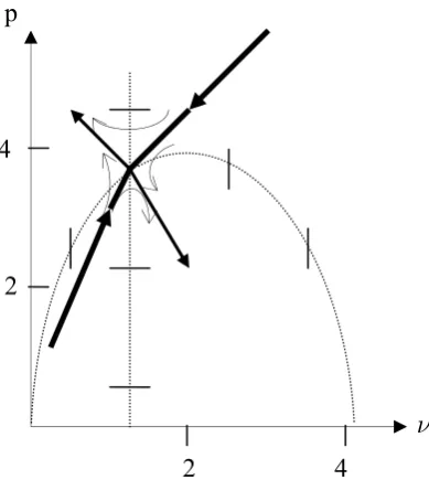
is a saddle point equilibrium.

The isoclines are q=ν

(

c−ν

)

for ν=0 and ν=c−₂ρ for q=0. The behavior inside

the sectors is given from the following Figure 2.

p

2

4

[image:10.595.144.343.178.386.2] [image:10.595.140.335.444.662.2]

ν 2 4

Figure 2.α Phase diagram for the system

( )

17 and

( )

18

p

4

2

ν

7. Concluding remarks

In this paper we show how methods of infinite horizon dynamic optimal control theory developed in the field of natural resource economics. We begin first with methodology analysis and second we propose two dynamical models of renewable resources.

As methodology suggests main variables involved in an optimal control problem distinguished in the states and controls. A state variable is the variable that only monitors the state of the economic system that transferred form an initial point time to the terminal time. Control variables are the chosen policy instruments that aid the motion of the state to made in an optimal way. One other variable involved at the solution process is the so called costate or auxiliary variable that is the shadow price of the state. The vehicle through the latter variable enters into the maximization process is the well known Hamiltonian function.

References

Benchekroun, H. and N.V. Long (2001) Tranboundary Fishery: A Differential Game Model, Economica, 69, 207 – 221.

Brock W.A. and D. Starrett (2003) Managing Systems with Non – convex Positive Feedback, Environmental and Resource Economics, 26, 575 – 602.

Dasgupta P. and G.M. Heal (1974), The optimal depletion of exhaustible sources. Review of Economic Studies, Symposium of the Economics of Exhaustible Resources, 3 – 28.

Dasgupta P. and K.G. Maler (2003) The Economics of Non – Convex Ecosystems: Introduction, Environmental and Resource Economics, 26, 499 – 525.

Dockner E.J., Jorgensen S. and Long N. V. – Sorger G. (2000) Differential Games in Economics and Management Science, Cambridge, Cambridge University Press.

Hotelling H. (1931), The economics of exhaustible resources, Journal of Political Economy 39, 137 – 175.

Levhari D, Mirman L. (1980) The great fish war. Bell Journal of Economics, 322-344.

Pontryagin et al (1961), The Mathematical Theory of Optimal Processes, Gordon and Breach Science Publishers (translated by K.N. Trirogoff)