A New Formula for Partitions in a Set of Entities into Empty and Nonempty Subsets, and Its Application to Stochastic and Agent Based Computational Models

(1)

A New Formula for Partitions in a Set of Entities into

Empty and Nonempty Subsets, and Its Application to

Stochastic and Agent-Based Computational Models

Ghennadii Gubceac, Roman Gutu, Florentin Paladi

Department of Theoretical Physics, State University of Moldova, Chisinau, Republic of Moldova Email: [email protected]

Received June 3, 2013; revised July 3, 2013; accepted July 10, 2013

Copyright © 2013 Ghennadii Gubceac et al. This is an open access article distributed under the Creative Commons Attribution Li- cense, which permits unrestricted use, distribution, and reproduction in any medium, provided the original work is properly cited.

ABSTRACT

In combinatorics, a Stirling number of the second kind S n k

 

, is the number of ways to partition a set of n objects into k nonempty subsets. The empty subsets are also added in the models presented in the article in order to describe properly the absence of the corresponding type i of state in the system, i.e. when its “share” . Accordingly, a new equation for partitions

0

i p 



,



P N m

type

in a set of entities into both empty and nonempty subsets was derived. The indis- tinguishableness of particles (N identical atoms or molecules) makes only sense within a cluster (subset) with the size . The first-order phase transition is indeed the case of transitions, for example in the simplest interpretation,

from completely liquid state to the completely crystalline state .

These partitions are well distinguished from the physical point of view, so they are ‘typed’ differently in the model. Fi- nally, the present developments in the physics of complex systems, in particular the structural relaxation of supercooled liquids and glasses, are discussed by using such stochastic cluster-based models.

0niN



1 , 2 0

L n N n 



typeC



n₁0,n₂ N



Keywords: Partitions; Agent-Based Models; Stochastic Processes; Complex Systems

1. Introduction

In mathematics, particularly in combinatorics and the study of partitions, a Stirling numbers of the second kind

 

, n

S n k k

    

  count the number of ways to partition a

set of n labeled objects into k nonempty unlabelled subsets. By the way, Stirling numbers of the second kind show up more often than those of first and third kind (or Lah numbers), and James Stirling himself considered this kind first [1]. Equivalently, they count the number of different equivalence relations with precisely k equivalence classes that can be defined on an n element set, and they can be calculated using the explicit formula

 

0

1

, 1

! k

k j n

j

k

S n k j

j k





 

  _{ }

 



, where k is the bi-

j

     

nomial coefficient. The sum over the values for k of the

Stirling numbers of the second kind, i.e.

0

n

n k

n B k 

 _

   



,

gives the nth Bell number, that is the total number of partitions of a cluster with n entities or agents [2]. The question arises when the empty subsets or clusters are needed to be used in the models, for example, with heterogeneous structure interactions and, subsequently, the partition by Stirling numbers of the second kind becomes inappropriate to count partitions in such complex systems [3].

In general, agent-based modeling is currently a tech- nique widely used to simulate complex systems in computer science and social sciences. On the other hand, a Markovian process is a stochastic process whose future probabilities are determined by its most recent values. The agent-based computational models (ABM) fits well this description, except for the cases when decisions are dependent on the state of the systems of more than one steps ago, which is the case when ABM agents experi- ence learning, adaptation, and reproduction [4].

(2)

populations, i.e. the partition process in a set of entities into empty and nonempty clusters, is derived and used to study how different behavioral norms affect the individ- ual and social welfare in a population with heterogeneous preferences. One can consider them as an idealization of an imperative and a more liberal approach to social norms or stylized behavioral rules studied by agent-based computational models [5,6]. Another application refers to the generic stochastic model for crystal nucleation which is useful to depict the impact of interface between the nucleus considered as a cluster of a certain number of molecules and the liquid phase for the enhancement of the overall nucleation process. It is generally known that first-order phase transitions occur by nucleation mecha- nism, and both the nucleus, a cluster of atoms or molecules, and the nucleation work, a energy barrier to the phase transition, are basic thermodynamic quantities in the theory of nucleation. However, the critical nucleus formation is statistically a random event with a probability largely determined by the nucleation work which in- creases with the subnuclei size [7]. The traditional differential equation modeling is not the alternative to agent-based models; only a set of differential equations, each describing the dynamics of one of the system’s con- stituent units, is an agent-based model [8].

The general formulation is outlined in Section 2. In Section 3 a probabilistic approach to the crystal nucleation process is considered. The main conclusions are presented in Section 4.

2. The Model

There are N entities which can be in 3 different states (call them left, center and right), and can play 3 actions (again left, center and right). Interaction in this agent- based model involves always one active and one passive

player, but agents can play both roles interchangeably. They have preferences over their states: accept one state, are neutral with respect to another state and reject the remaining state. When two agents meet, the active player sets the passive player’s state according to his action,

which in turn is determined by one of the applied rule. This identifies only 6 possible combinations. Denote with 1 6 the shares of the population characterized

by each combination of preferences, as in Table 1. That is, drawing randomly one agent, it will be of type i with probability i. After each interaction, the passive player gets a payoff of +1 if it is in the accepted state, a payoff of 0 if it is in the neutral state, and a payoff of −1 if it is in the rejected state. The active player does not get any feedback. If the active player follows the first J-rule, it always plays the action corresponding to the accepted state. If it follows the second H-rule, it randomizes between actions corresponding to the accepted and neutral states. The further example will clarify. Suppose two individuals, A and B, meet. Player A is the active one, and rejects left, accepts right, and is thus neutral with respect to the center. Player B is the passive one. It accepts left, rejects right, and is neutral with respect to center, like player A. Suppose A follows the J-rule, and will play right, setting B’s state to right. B will then have a payoff of −1. Suppose, on the other hand, that A follows the H-rule, and will randomize between center and

right. The payoff for B could then be either 0 or −1. Note that there is no strategic interaction in the model: the passive player’s payoff depends on the active player’s choice, but the active player’s choice does not depend on the passive player in any way, so the game-theoretic solution concepts like Nash equilibrium become useless.

pp

p

Aggregate results are defined in terms of both the mean π and the variance σ2_{of the payoffs which denote}

the stability and the heterogeneity of population, respect- ively. However, in order to avoid arbitrary choices we do not specify a particular functional form, and report sepa- rately the results for the mean and the variance. Let

1, 2, ,

N   be the total number of entities in the model, and the



n n n n n n1, , , , ,2 3 4 5 6



is their partition

into m6 subsets. Each subset can be called cluster, and the process itself—clustering. The size of each cluster can vary from 0 to N, ni 0, ,N i1, 6, and

6 1 i

i

n N



[image:2.595.55.540.609.737.2]



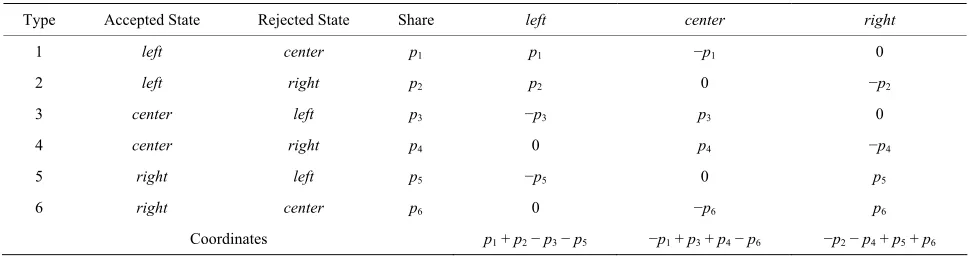
. The number of possible partitions P is a

Table 1. Distribution of preferences in the heterogeneous system with 6 types of states.

Type Accepted State Rejected State Share left center right

1 left center p1 p1 −p1 0

2 left right p2 p2 0 −p2

3 center left p3 −p3 p3 0

4 center right p4 0 p4 −p4

5 right left p5 −p5 0 p5

6 right center p6 0 −p6 p6

(3)

function of N and m, and the explicit solution is



















 











2

6 1 6 2 6 3

2

3 3

2

6 4

2 2

4 3 1 4 4

2 3

6 5

2 3 2 2 2

5 4 2 3 5 4 2 3 2 1 , 6 1 1 3 2 1 3

5 4 3

4 N

i

N N

i i

N N i N N

i i l i i

N N

i i

N N

i l i i

P N m

C N C i C

N N i i C

i i l N i i C

N N i i N i i l

i l N i i

                                _ _     _     _      _                



 

  



 



 



















1 2 i l  



 





5 6 6 2 5 2

5 5 5

2 3 4

2 2 2

4 1 5 4

2 2

3 2 2 1

5

1

2 74 213 2 11 13

2 1 3 2

3 1 _, 5! N N i

N N N

i i i

N i N N

i l i l i

i

C

N N i

N i N i i

N i i l i l

N i                                         



  



where 6 1 6 5 6 2 6 4 6 3 6 6

are combinations given by the binomial coefficient

6, 15, 20, 1

C  C  C  C  C  C 



!



! ! m k

m m

C

k m k k

  _{ }



  . In general, when the number

of subsets , the number of possible partitions P of

N agents into mm subgroups or subsets is 1





_{   }

1

1 1 , 1 ! m i

P N m N i

m 









1

P m 

5

m

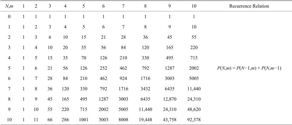
N is given by 330 210 120  , where 210 is the number above and 120 is the number on the left of 330. The diagonal elements of the bi-triangular array of values for the numbers of partitions are 1, 2, 6, 20, 70, 252, 924, 3432, 12,870, 48,620, …, and it is represented by nth central binomial coefficient:





 

2 2 ! 2 2 , ! n n C n n

n _n

  _ _

  for all n0.

They are called central since they show up exactly in the middle of the even-numbered rows in Pascal’s train- gle. These numbers have the generating function

2 3 4

6 7

1 _{1 2} ₆ ₂₀ ₇₀ ₂₅₂

1 4

924 3432 .

5

x x x x

x x x           x

It is known that the asymptotics for the central binomial coefficient C n n



2 ,



can be written in the form of a particular case of the Wallis formula, i.e.

[image:3.595.56.538.528.734.2]

 

2 4 2 2 2 lim lim 2 1 2 n n n n n n n n n              _ _       _ _     ,

Table 2. Bi-triangular array of values for the numbers of partitions P(N,m).

N,m 1 2 3 4 5 6 7 8 9 10 Recurrence Relation

0 1 1 1 1 1 1 1 1 1 1

1 1 2 3 4 5 6 7 8 9 10

2 1 3 6 10 15 21 28 36 45 55

3 1 4 10 20 35 56 84 120 165 220

4 1 5 15 35 70 126 210 330 495 715

5 1 6 21 56 126 252 462 792 1287 2002

6 1 7 28 84 210 462 924 1716 3003 5005

7 1 8 36 120 330 792 1716 3432 6435 11,440

8 1 9 45 165 495 1287 3003 6435 12,870 24,310

9 1 10 55 220 715 2002 5005 11,440 24,310 48,620

10 1 11 66 286 1001 3003 8008 19,448 43,758 92,378

P(N,m) = P(N−1,m) + P(N,m−1)

(4)

where (x) is the gamma function, so

2_n _~ 4n _, n

n n

 

   

  .

By the way, this equation can also be used to deter- mine the constant 2 in front of the Stirling’s formula.

Now it is straightforward to see that when all individuals share the same preferences (polarization) the first rule gives a higher payoff. In the other extreme case, when preferences are equally distributed in the ensemble

(dispersion) and 1 2 6

1 , 6

p  p  p  it is again

straightforward to see that the rules are equivalent, and lead to an average payoff  0



N

. Consider next an active

player of type 1 (accepts left and rejects center) which meets in turn all other (passive) agents, including himself. If it follows the first rule, then it will play left causing a payoff of +1 in 1 2 agents, and a payoff of −1

in 3 5 agents. Note that there are

similar entities in the ensemble. Suppose now that everybody meets everybody else both as active and as pas- sive players. Coupling them randomly and randomly choosing active and passive players only adds some noise to the simulation results. So the average payoff when everybody plays according to the first J-rule is



p p





p p N



p₁p N₂

















1 1 2 1 2 3 5

3 4 1 3 4 6

5 6 2 4 5 6 .

p p p p p p

     

     

     



(2)

Similarly, the average payoff with the second H-rule is

















2 1 1 3 5 6

2 2 3 4 5 3 1 3 5 6 4 1 2 4 6 5 2 3 4 5 6 1 2 4 6

1 2

.

p p p p p

p p p p p p p p p p

p p p p p p p p p p

p p p p p

    

        

         

   



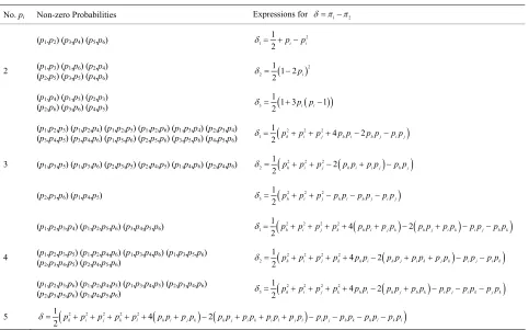
(3)

To study the behavior of  ₁ ₂ based on Equations (2) and (3), it is convenient to set some of the probabilities to zero. It is straightforward to see that when there is just one probability different from 0 (and thus equal to 1)

we have ₁ ₂ 1 0 2

    . In general, the number of different possible combinations of non-zero probabilities is given by the above binomial coefficient m k.

Thus for two non-zero probabilities we obtain a set of

6 2

C

15

C  equations which can be grouped in just 3 different functional forms shown in Table 3. Figure 1

[image:4.595.57.222.87.131.2]

graphs these 3 curves for all values of pi and pj  1 pi. The J-rule still performs better in all cases but one, when

Table 3. Expressions of π1π2 for different numbers of non-zero probabilities pi, i = 1, 2, ···, 6.

No. pi Non-zero Probabilities Expressions for    1 2

(p1,p2) (p3,p4) (p5,p6) 1 2

1

2 pi pi

   

(p1,p3) (p1,p6) (p2,p4)

(p2,p5) (p3,p5) (p4,p6)  

2 2

1 _{1 2}

2 pi

  

2

(p1,p4) (p1,p5) (p2,p3)

(p2,p6) (p3,p6) (p4,p5) 3



 



1

1 3 1

2 p pi i

   

(p1,p2,p3) (p1,p2,p4) (p1,p2,p5) (p1,p2,p6) (p1,p3,p4) (p2,p3,p4)

(p3,p4,p5) (p3,p4,p6) (p1,p5,p6) (p2,p5,p6) (p3,p5,p6) (p4,p5,p6)





2 2 2 1

1 ₄ ₂

2 ph pi pj p ph i p ph j p pi j

      

(p1,p3,p5) (p1,p3,p6) (p2,p3,p5) (p2,p4,p5) (p1,p4,p6) (p2,p4,p6) 2



2 2 2





1

2

2 ph pi pj p ph i p pi j p ph j

      

3

(p2,p3,p6) (p1,p4,p5) 3



2 2 2



1

2 ph pi pj p ph i p ph j p pi j

      

(p1,p2,p3,p4) (p1,p2,p5,p6) (p3,p4,p5,p6) 1



2 2 2 2









1

4 2

2 ph pi pj pk p ph i p pj k p ph j p pi k p pi j p ph k

          

(p1,p2,p3,p5) (p1,p2,p4,p6) (p1,p3,p4,p6) (p1,p3,p5,p6)

(p2,p3,p4,p5) (p2,p4,p5,p6)





2 2 2 2 2

1 ₄ ₂

2 ph pi pj pk p ph i p ph j p pi k p pj k p pi j p pi k

          

4

(p1,p2,p3,p6) (p1,p2,p4,p5) (p1,p3,p4,p5) (p2,p3,p4,p6)

(p2,p3,p5,p6) (p1,p4,p5,p6)





2 2 2 2 3

1

4 2

2 ph pi pj pk p ph i p ph j p ph k p pi j p pi k p pj k

          

5 1



2 2 2 2 2 ₄



 

₂



2 ph pi pj pk pl p ph i p pj k p ph j p pi k p pi l p pj l p pi j p ph k p ph l p pk l

[image:4.595.59.542.432.733.2]

(5)

0.1 0.2 0.3 0.4 0.5 0.6 0.7 0.8 0.9 1 0.1

0.2 0.3 0.4 0.5 0.6 0.7

π1 – π2

[image:5.595.152.445.82.265.2]

pi

Figure 1. π1π2 in the case of two non-zero probabilities, pi and pj = 1 − pi. the two rules are equivalent. However, from three non-

zero probabilities onward things start to look differently. For three non-zero probabilities we have 6C320

equations, while for four non-zero probabilities there are equations, and for five non-zero probabilities

6 5 equations. These equations reduce to just three

different functional forms in case of three and four non- zero probabilities, and to just one expression in case of five non-zero probabilities.

6C4 15

6

C 

A trend towards a better performance of the H-rule, as the distribution of preferences inthe system becomes less polarized, is evident. However, in order to better investi- gate it, adefinition of how much preferences are polarized is needed.We represent the distribution of states as a single point in a three dimensional space, where the axes are labeled l, c and r. The l coordinate is found by counting all agents who accept left, and subtracting all agents who reject left. The result is then normalized to the size of the population. Similarly for the other two coordinates. Hence,

1 2 3 5

3 4 1 6

5 6 2 4

, , ,

l p p p p

c p p p p

r p p p p

   

(4)

where . Note that different distributions of states can lead to the same point in the sphere. For in- stance, the point in the origin is given not only by

0

l c r  

1 2 p6 1 6

p p  , but by any combination of preferences such as p1 p3, p2 p5, and 4 6. Tak-

ing into account Equation (4), one can define now the polarization of states as the distance from the center of the sphere:

p  p









2 2 2

1 2 6

, , , , ,

d l r c d p p  p  l r c . (5) Note that d_{ }0, 2

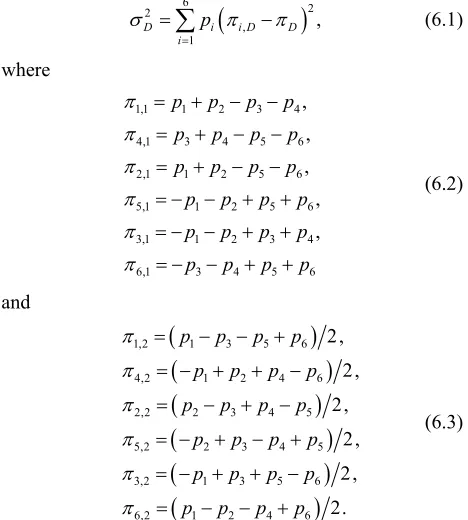
The variances 2 1

 and 2 2

 are defined for each dis- crete distribution D1, 2 with the expectation (mean) value D as follows:



6 ₂

2

, 1

,

D i i D D

i

p

  









(6.1) where

1,1 1 2 3 4 4,1 3 4 5 6 2,1 1 2 5 6 5,1 1 2 5 6 3,1 1 2 3 4 6,1 3 4 5 6

, , , , ,

p p p p

     

   

    

(6.2)

and

























1,2 1 3 5 6

4,2 1 2 4 6

2,2 2 3 4 5

5,2 2 3 4 5

3,2 1 3 5 6

6,2 1 2 4 6

2, 2, 2,

2, 2, 2.

p p p p

     

   

    

   

    

    

   

(6.3)

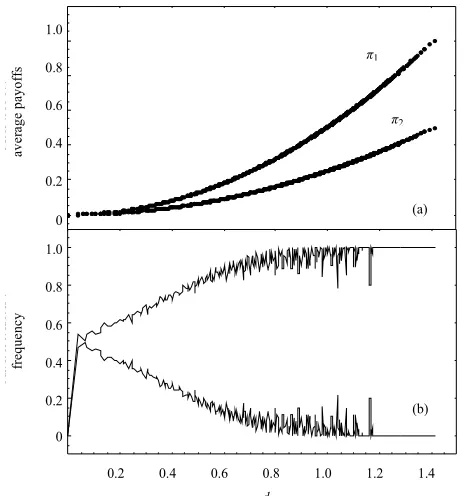
Figure 2 explores how outcomes vary as functions of the distance d l r c



, ,



defined by Equation (5). The whole range

 

0,1 is sampled, for all probabilities

1 6. The step considered for creating all combina-

tions of probabilities is 0.025, i.e. the total number of agents is 40. The average values for 1

pp

 and 2 are

shown in Figure 2(a), and for each value of the distance from the center of the sphere, , the frequency of wins with each rule is computed (see Figure 2(b)). When 1 2



, ,

d l rc



0

  

1 2 0

a win is assigned to the first J-rule, and when    a win is assigned to the second



: all points thus lie inside a

[image:5.595.307.541.333.593.2]

(6)

0.2 0.4 0.6 0.8

1 1.2 1.4

d

0

0.2

0.4

0.6

0.8

1 sff

oy

aP

0.2 0.4 0.6 0.8

1 1.2 1.4

d

0

0.2

0.4

0.6

0.8

1 yc

ne

uq

erf

d

0.2 0.4 0.6 0.8 1.0 1.2 1.4 (b) (a)

av

er

age pa

yof

fs

fre

que

nc

y

1.0

0.8

0.6

0.4

0.2

0 1.0

0.8

0.6

0.4

0.2

0

π1

[image:6.595.56.288.82.330.2]

π2

Figure 2. Average values for (upper line) and (a), and relative frequency of negative and positive values for

(b) as functions of the distance d p from the center of sphere with a radius of

1

π π2



1, ,p2 1

π π2 ,p6



2: 40 entities, 6 clusters in a similar ABM model.

one. Exactly in the center of the sphere the two rules lead to the same payoff, independently of the underlying distribution of states. Close to the center, each rule wins in about 50% of the cases. Then, as we move away from the center, the first rule improves its performance, and it is always better when the states are totally polarized, but the total number of states for intermediate values of the distance d is much larger than for the dispersed and polarized states.

Meanwhile, the variance (6.1) with the J-rule (6.2) is generally higher than the variance with the H-rule (6.3), especially when the preferences are dispersed in the system, and when they are quite polarized. On average, however, when one rule is better in terms of higher ex- pected payoffs it is also better in terms of lower heterogeneity, and there are the same average values of the scale-free coefficients of variation on the distance d for any level of fragmentation of states.

3. A Probabilistic Approach to the Crystal

Nucleation Process

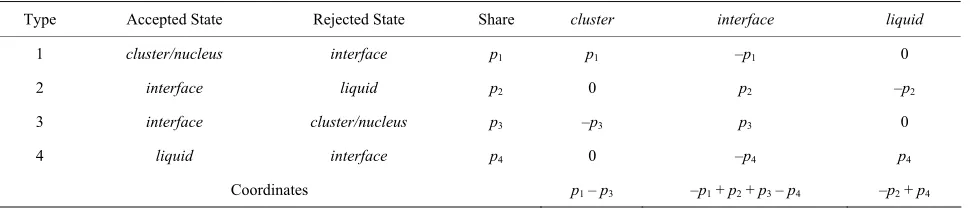
The second application refers to the nucleation process, a widely spread phenomenon in both nature and technol- ogy, which may be considered as a representative of the aggregation phenomena in complex systems. Let’s consider N atoms which can be in 3 different states (cluster,

liquid and their interface), and can perform 4 possible moves: liquid to interface, interface to liquid, interface to

cluster, and cluster to interface. One can identify 4 different combinations denoted with probabilities 1 4,

as in Table 4. That is, drawing randomly one particle, it will be of type i with probability i Let

pp

1, 2, ,

p N   

be the total number of atoms in the system, and



n n n n1, , ,2 3 4



are their partition into 4 subsets. Each subset can be called cluster, and the number of possible partitions (1) in this case is





3





1

, 4

3!i

P N m N i



 

_

 ,

where ni 0, ,N i1, 4 and



. For example, in

a system of N=1000 atoms, P N m



, 4



equals to

4 1 i

i

n N



167,668,501! Accordingly, the n eated computer runs in an ABM model would be very large due to different possible partitions. But we are able to overcome this problem, as already mentioned in the previous section, by developing similar stochastic mathematical models which can describe exactly the results of the agent- based computational models, and, finally, by bridging the gap between ABM modeling and stochastic processes.

Let’s consider further that each particle interacts wi umber of rep

th the entire group both as an aggressor in terms of the Kolmogorov mathematical theory [9], and as a passive agent in terms of the ABM computational models as well. Then the mean π, namely the stability index, takes here the form



 









1 1 3 2 3 1 2 3 4 4 4 2

p p p p p p p p

p p p

      

 

p



(7.1)

or, taking into account that , one can exclude

one probability, for example p4, from the above equation:

4 1

1 i i

p 









p p p

  











1 1 3

1 2 3 1 2 3

2 3 2 3

1 2 1

1 2 2 .

p p p p p p

p p p p

      

    



(7.2)

One can represent again the distribution of states as a three-dimensional point



l r c, ,



inside a sphere, and the mean payoff π (Equation r Equation (7.2)) can be obtained as a function of the distance

(7.1) o









2 2 2

1 2 3 4

, , , , ,

d l r c d p p p p  l r c , where the axes are labeled l, c and r l:  p1p3,

2 3 1 4, 4 2

c p p p p rp p , and, as stated in the previous section, l c r  0 and d_{ }0, 2_. Thus

different distributions e point

in the sphere, i.e. different microscopic partitions can

(7)

rejected states in the system.

[image:7.595.58.543.102.206.2]

Type Accepted State Rejected State Share cluster interface liquid

Table 4. Distribution of accepted and

1 cluster/nucleus interface p1 p1 –p1 0

2 interface liquid p2 0 2 2

3 3 3

4 – 4 4

Coordinates p1 – p3 –p1 + p2 3 – p4 –p2 p4

p –p

3 interface cluster/nucleus p –p p 0 4 liquid interface p 0 p p

+ p +

enerate the same result on aggregate inside a sphere g

around the origin. The results for the two limit cases are obviously: if all particles would show the same behavior, then d  2 and there is a maximum stability of states in such a completely asymmetrical system, but  0

for a homogeneous system, p1p2 p3 p4 ,

and for combinations such as

1 4

1 3

p p and p2 p4 in

the case of unstable states.

4. Conclusions

ls developed in this paper were used

between agent-ba

its diagonal elements are represented by nth central bi-

e point inside the sphere around th

ardi for his ABM contribu-

REFERENCES

[1] R. L. Graham tashnik, “Concrete

Mathematics. ce,” 2nd

Mathematical mode

together with agent-based computations to study interactions in two quite different heterogeneous systems. The models are general ones and allow simulations for any size of the system. Our results also support the idea that general properties observed in the complex systems of any kind, which arise from the interplay between random interactions and their complex structures, could be suc- cessfully investigated by the same tool. For example, these properties are frequently found in the physical sciences, and are the domain of non-equilibrium statistical mechanics. Because of the real limitations in the use of analytical methods to study such problems, it is often necessary to resort to numerical ones, and the advent of computer simulations has led to an increase of scientific activity in this area that has emerged nowadays as a ma- jor subject of interdisciplinary research.

The recent discussions about the gap

sed computational models and stochastic analytical models have stimulated the research on this topic [3,10]. In such context, the article supports a unified probabilistic approach to simulation of multi-agent interactions in heterogeneous complex systems. This method appears phenomenological if it is not agent-based, and we prove analytically that the average outcomes of multiple agent- based computations can be described precisely. Further- more, a useful aggregation procedure for representing the three-dimensional distribution of states, and a general formula that describes clustering process among inter- acting agents in heterogeneous populations, which is the Equation (1) for partitions in a set of entities into empty and nonempty subsets, are proposed. Bi-triangular array of values for the numbers of partitions is presented, and

nomial coefficient.

In particular, we obtained that different distributions of states can lead to the sam

e origin, i.e. different microscopic partitions can gener- ate the same aggregate result. It would be a particular conclusion set for the analyzed situations, but one would expect this in different circumstances due to the universal aspects observed in the behavior of complex systems.

5. Acknowledgements

F.P. thanks Dr. Matteo Richi tion.

, D. E. Knuth and O. Pa

A Foundation for Computer Scien Edition, Addison-Wesley Professional, Reading, 1994. [2] J. Sandor and B. Crstici, “Handbook of Number Theory

II,” Kluwer Academic Publishers, Dordrecht, 2004. http://dx.doi.org/10.1007/1-4020-2547-5

[3] F. Paladi, “On the Probabilistic Approach to Hetero ous Structure Interactions in Agent-Based Computational gene- Models,” Applied Mathematics and Computation, Vol. 219, No. 24, 2013, pp. 11430-11437.

http://dx.doi.org/10.1016/j.amc.2013.05.042 [4] E. Bonabeau, “Agent-Based Modeling

chniques for Simulating Human Systems,” : Methods and Te- Proceedings of the National Academy of Sciences of the United States of America, Vol. 99, No. 3, 2002, pp. 7280-7287. http://dx.doi.org/10.1073/pnas.082080899

[5] M. Richiardi and F. Paladi, “Jesus, Hillel and the M the Street. Moral and Social Norms in Heterogeneous an of

,” European Journal of Economic and

2nd Edi- Populations,” LABORatorio R. Revelli Working Paper 40, 2005.

http://eco83.econ.unito.it/terna/swarmfest2005papers/rich iardi_paladi.pdf

[6] M. Richiardi, “Jesus vs Hillel. From Moral to Social Norms and Back

Social Systems, Vol. 19, No. 2, 2006, pp. 171-190. [7] D. Kashchiev, “Nucleation. Basic Theory with Applica-

tions,” Butterworth-Heinemann, Oxford, 2000.

(8)

tion, Springer-Verlag, Berlin, 1985.

[9] A. N. Kolmogorov, “On Statistical Theory of Metal Crys- tallisation (in Russian),” Izvestiya Academy of Sciences

205013109 ,

“L

USSR, Mathematics, Vol. 3, 1937, pp. 355-360.

[10] L. Feng, B. Li, B. Podobnik, T. Preis and H. E. Stanley,

inking Agent-Based Models and Stochastic Models of Financial Markets,” Proceedings of the National Acad- emy of Sciences of the United States of America, Vol. 109, No. 22, 2012, pp. 8388-8393.