Sensors Grouping Model for Wireless Sensor Network

(1)

http://dx.doi.org/10.4236/jst.2013.34020

Sensors Grouping Model for Wireless Sensor Network

*

Ammar Hawbani, Xingfu Wang, Yan Xiong

School of Computer Science and Technology, University of Science and Technology of China, Hefei, China Email: [email protected]

Received November 6, 2013; revised December 6, 2013; accepted December 13, 2013

Copyright © 2013 Ammar Hawbani et al. This is an open access article distributed under the Creative Commons Attribution License, which permits unrestricted use, distribution, and reproduction in any medium, provided the original work is properly cited.

ABSTRACT

The grouping of sensors is a calculation method for partitioning the wireless sensor network into groups, each group consisting of a collection of sensors. A sensor can be an element of multiple groups. In the present paper, we will show a model to divide the wireless sensor network sensors into groups. These groups could communicate and work together in a cooperative way in order to save the time of routing and energy of WSN. In addition, we will present a way to show how to organize the sensors in groups and provide a combinatorial analysis of some issues related to the performance of the network.

Keywords: Sensors Groups; WSN; Sub-Group; Sensors Organize

1. Introduction

A wireless sensor network consists of spatially distributed autonomous sensors to monitor physical or environ- mental conditions, such as temperature, sound, pressure, etc. [1-5]. The sensors cooperate with each other to mon-itor the targets and send the collected information to the base station [6-8]. Sensors are battery-powered devices having a limited lifetime, restricted sensing range, and narrow communication range [9-11], and densely de-ployed in harsh environment [12-15]. Organization of sensors in the form of groups is very important, which would facilitate transferring data and routing from one group to another, and it also offers an easy way to analyze the WSN problems such as coverage, localization, connectivity, tracing and data routing [16-20].

2. Sensors Grouping Strategy

A Group of sensors is a collection of overlapped sensors in a single area. Let us define the degree of overloaded sensors by the maximum number of sensors overlapped in the same area, here we denote to the maximum coverage degree of an area by



, 1, ,



r i i k

D  s s  s x

where x0,1, 2,, ,k where is an area notation

called r, 1

r

D

, ,

i i k

s s  s are the overlapped sensors, and x the number of overlapped sensors. The overlapped sensors that create a degree of an area



,si1, ,sk



r i

D  s  k Create a group of sensors denoted by



, 1



k i i

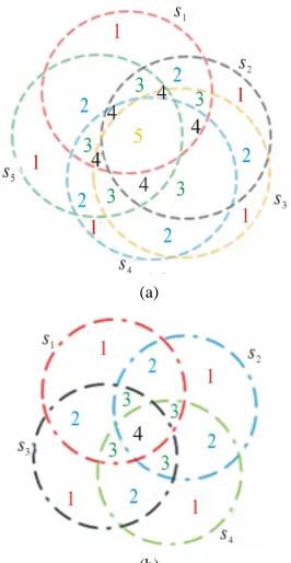
G  s s_,,s_k we call the coverage degree. Figure1 shows four groups 1 2 3 and G4.

The maximum degree of sensor 2

k

, ,

G G G ,

s and senor s3 is



1,s2



2

r

D  s  that occurs in the area of intersection, which means that there is one and only one area covered by two sensors and that is the maximal overlapping that could be produced, so sensor s2 and s3 create a group

of two sensors denoted by 2 _





1 2 . Sake of con- venience, we denote to the group of sensors that build up the WSN by

,

G s s







 



*

G G

k

2 3 4

,G G,

  s s₂, ₃ , s1,s3,s4 , s1,s4,s5,s6 ,

which we call it the mother network group or simply the mother group.

2.1. Counting the Sub-Areas of Sensors Group

Here we start by asking, how many sub-areas are gener-ated if unit disk sensors are partially overlapped? As- suming there is no fully overlapping between sensors, and all sensors are homogenous (sensors have the same sensing range). Say F k

 

is the function to count the number of sub-areas, definitely F

 

0 0. F

 

1 1,

 

2 3

F  , F

 

3 7, F

 

4 13(see Figure 2). What is F k

 

? k1.

*_{This paper is supported by The National Natural Science Foundation}

of China (NO.61272472, 61232018, 61202404) and the National

(2)

(a)

[image:2.595.107.238.82.390.2]

(b)

Figure 1. Partitioning the WSN into group.

k

G is







1

1 1

2 k

i

k

k i k k





 

_{ }    

 



1





(1) Proof: suppose we have a group of sensors

as shown in Figure 3, we can see that the number of areas inside each sensor’s range is seven. Using Top-down approach from 1



4

1, 2, 3, 4 G  s s s s

s to s4, the

number of areas for the top sensor

 

s1 is seven (red areas namely 1, 2, 3, 4, 5, 6, 7). The number of areas inside the sensor’s range s2 are seven, namely (4, 5, 6,

7, 8, 9 10), but the red colored areas, 2, 3, 4, 5, already counted in s1, so there are only 3 blue colored areas

inside sensor’s range s2, namely 8, 9, 10. For the sensor 3

s , it has seven areas inside its sensing range, the 3, 5, 6, 7 are red areas already counted in sensor’s range s1, the

area 10 is blue area already counted in sensor’s range s2,

thus still two black areas in sensor’s range s3, namely

11, 12. For sensing range of s4, there are seven areas

inside it, three are red areas (4, 5, 6), two are blue areas (9, 10), and one area is black (11), so there is still one area only in s4 (13). Therefore, the number of areas

from top to down is 7 + 3 + 2 + 1 = 13. Generally, counting the sub-areas from top to down, the top sensor contains

1 2

k

      

Figure 2. (a) the number of sub-areas of (b) the num-ber of sub-areas of (c) the number o -a as of

1

G f sub 2

G re 3

G (d) the number of sub-areas of 4

[image:2.595.350.498.83.233.2]

G .

Figure 3. The 13 areas of group

contains

4

G .

1

areas, the second sensor inside the group

k areas, the third sensor contains k2

areas… the last sensor contains one area



k



k1



. Totally, th re



 







1 1 2 1

2

k

k k k k

 

ere a

_{ }      

   of areas. Gen -

erally, there count of areas is

 

























1 1

1

2 i

F k



 _{ }

 



1 !

1

2! 2 ! 2

1 1

1

2 2

1 1

k

k i k k k

k

k k k k

k k 

 



  



 

  

  

In addition, we can proof theorem 1 by counting the areas of a group basing on the degree of coverage, if an area covered by k sensors then it called k-covered area. For a group Gk there is only one area is k-covered (the maximum degree of coverage), in the remainder areas, there are k areas are1-covered, k areas are 2-coverd, k areas are 3-coverd… k areas are k-1 covered. Let kj be

[image:2.595.362.486.291.392.2]

(3)





5

1, 2, 3, 4, 5

G  s s s s s , the number of 1-coverd areas is five. can count the of areas of sensors group

k

G as below

 

1

k k i i

F k We

:

sum

 





 





1 2

1 1

k k

F k

k k k k k

  

  

       



Lemma 1: for sens there are only one area eas are 2-coverd, k co

rage for eac tio

a Sensors Gr

deno

3

1 time

1 s

k k

k

K



  



or range belo s to a group k-covered, k area 1-coverd, areas are 3-coverd… and k areas k-1

h area, the number of intersec-

oup

ped sensors ing, here we tersection points by

ng Gk,

k ar-vered.

Lemma2: for a group Gk, all sensors have the same characteristics, for example, the number of areas, the degree of cove

n points located on the border of the sensor, and the number of intersection points located inside sensor’s range.

2.2. Counting the Intersection Points of

Counting the intersection points of k-overlap is an easy combination problem. Before prov

te to the number of in P k

 

, clearly P

 

0 0 , P

 

1 0 , P

 

1 0 , P

 

2 2 ,

 

3 6

P  , P

 

4 12… then what is the P k

 

? k2 Theorem2: the number of intersection points o -sors gro

f sen up Gk is

 



1



P k k k (2) Proof: Assuming t

sensor has two inte

sensor, since each sensor has

hat there are k sensors and each rsection points with each neighbor





2 k1 intersection points with others, applying this method to all sensors, we get the total amount of intersection points as 2k k



1



. However, while calculating, ev gle point has been repeatedly counted twice, thus the right answer in regards to the intersection points quantity should be



ery sin



1

k k  . We can use top down approach to calculate the num-ber of intersection points, as shown in the Figure 5(a)





5

1, 2, 3, 4, 5

G  s s s s s . s1 is the top sensor; s5 is the

bo

range of the top sens

ttom sensor of the group. The number of intersection points inside (internal) and on the border of sensing

or



s1



is



k1



k2



. In the second node



2



2

s , there are k-2 of intersection points. In the third node

 

s3 , there are k-3 of intersection points. In the fourth node



s4



, there section points, and th is 0 intersection points in the bottom sensor.

Totally the number ntersection points is

 

are k-4 of inter ere



1



2



_

_

_

_

1 k

k k

P k   k i k k

2

2 i

 



  

Another method to count the intersectio points of a n group, we can imagine that the number of intersection points as the number of 2-permutation of k sensors, for example, S is a set of overlapped sensors



1, 2, 3, 4



S s s s s . The 2-permutation of S is:



s s1, 2



,



s s1, 3

 

, s s1, 4



,



s s2, 1



,



s s2, 3

 

, s s2, 4



,



s s3, 1

 

, s s3, 2

 

, s s3, 4



,



s s4, 1

 

, s s4, 2



,



s s4, 3



   















! , 2

2 !

1 2 !

where 1 1

2 !

k P k

k

k k k

k k

k

 

 

   

 k

We can use the Recurrence relation to find the ber of intersection points of a group of sensors. We can find the recurrence relation of the number of intersection points as

num

below:

 



1

 

2 1



f n f n n

 

0

1 0

P k n f

   

  _ 

 _



(3)

which can be easily solved using generatio

[21]. (See the proof of theorem 3), the solution is n function



1



0 0 0

n n c c  , so P n

 

n n



1



.

That Located within the Sensing Rang of a Sensor Associated to a Group (Internal

In F f

inter 5, in

Figu section points lo-

2.3. Counting the Number of Intersection Points

Points and External Points)

igure5(c), we can see that when k = 3 the number o section points located in the black sensor are

re5(b)k = 4, the number of inter

cated in the red sensor are 9, when k = 5 the number of intersection points are 14.

Theorem3: for a group of sensors Gk, the number of intersection points within the sensing range of sensor is

  

k1



2





k1



1

2 2

k i

k k

E s    

Proof: it is easy to realize tha the numt ber of intersec -tion points (internal and external) of the sens is satis-fying the recursive relation:

or

 





of i f

 

2 2

1

2

n i

f n n f n

E s n

   

 _ 

(4)

(a)

(b)

Figure 4. (a) group of sensors, (b) group of sen-sors.

5

G 4

G

(a) (b)

(c)

Figure 5. (a) Intersection points of group , (b) intersec-tion points of group , (c) intersection ints of group

e r ppose the generation function is

5

G po 4

G

3

G .

So finding the solution to this recursiv elation is the proof of the theorem.

Su

 

0

n

A x f n x







In addition, suppose that f

 

0 2

 





 





0 1

1 1

0 0

0 1

1

n n



A x f f n x f n n x

x nx

x f n x nx

 

 

 

 

    



 



f n

 









 





2

1

x A x xA x

x

  



 





3

2

1 ₁

x A x

x _x

 

 

 



1



1

2

n i

n n E s   

The external intersection points of sensors are the points located on the border of a sensor. However, the internal points are those points located inside the sensors but not on the border.

Lemma 3 (the number of external points): the number of intersection points located on the border of a sensor, which belongs to a group of sensors Gk is

 

2



1



k i

B s  k .

Proof: from Figure 5, it is easy to realize that the number of intersection points (external) of the sensor is satisfying the recursive relation:

 

2 ( 1)

f n  

 

2

2 2

n i

B s n

f

  

 _



f n 

We can solve this relation using generation function as in the proof of theorem 3. Therefore, the solution to this recursive relation is the proof of this theorem

 

2



1



n i

B s  n .

Lemma4 (the number of internal points): the number of intersection points located inside a sensor (not includ-ing the points located on the border) is

  

1



2



2

k i

Proof: from Figure 5, it is easy to realize that the number of intersection points (internal

k k

W s 

) of the sensor is satisfying the recursive relation:

 





1 2

f n  n f n  

 

3

3 1

n i

W s n

f

  

 _



(5)



We can solve this relation using generation function as in the proof of theorem 3. Therefore, the solution to this recursive relation is the proof of this theorem.

 



3



1, 3

2

n i

n n

W s    n

[image:4.595.104.237.83.340.2] [image:4.595.328.521.86.269.2]

(5)

From lemma 3, and lemma 4, we get the number of in-tersection points of a sensor that belongs to a group of sensors G E sn n

 

i by counting the intersection points

located border of the sensor (external points) and the intersection points located inside the s nternal po on the ensor (i ints).

 





 













_

_













2 2 2 2

3 2 4 1

2

3 2 4 4

2

1 2

1 1

2 2 2

i n si

n n n

n n n

n n

n n n n

                     (6) 2.4. Counting the Number of Areas within the

Sensing Range of a Sensor That Belongs to a Group

G

k

Theorem 4: e number of areas inside the sensor

3

1 2 1

2

3 2

2 1

n n i

n n

E s W B s n

n n n                _ _ 

Th si

that belongs to a group of sensors Gk is

 





 

1 , 2

2

k i

k Q s   _{ } k

  1 1 2 k i k k

Q s   

1 2

k i

P k Q s  

Proof: it is easy to realize that the number of areas in-side the sensor is satisfying the recursive relation:

 





 

1 1

1

n i

f n n f n

Q s n

1 1 f          _ 

We can solve this relation using generation func (7)

tion as in the proof of theorem 3. Therefore, the solution to this recursive relation is the proof of this theorem

 

1



1



2

n i

n n Q s   

2.5. Counting the Number of Areas Located within the Sensing Range of a Sensor That Belongs to Multiple Groups

In Figure1, the network sensors group is:





  

 



* 1 2 3 4

0 2 3 1 3 4 1 4 5 6

, , ,

, , , , , , , , ,

G G G G G

s s s s s s s s s s

 

Our goal is to count the number of areas inside t or i

he sens s that associated to multiple groups. The groups

hich i

to w s belongs can be defined as following: an define the mother grou

Say that s_iG G Ga, b, c then we c p of si as:







 



*

,

, ,

a _{G G}b c _s

 _i   _i , _i, , _i

G G s  s .

, where a, b, c are the positive integers

i i i

, , ,

a b c

i i i i

s G G G  nu



mbers that represent the degree of coverage.

As shown in Figure 1 we can define the mother group of sensors s0, s1, s2, s3, s4, s5 and s6 as below:

1

Since s0G only e mother group of sensor

0

, then th s is G0*

 

G10 

 

s0

Si ce n s1G G3, 4, then the mother group of sensor

is





1

s * 3



 



1 1

G  G G4

1  s s s1, 3, 4 , s s s s1, 4, 5, 6

Since 2 2

,

s G , then the mother group of sensor s2 is

 





* 2

G2 G2  s s2, 3

Since s3G G2, 3, then the mother group of sensor

3

s is G3*



G G2, 33







s s2, 3

 

, s s s1, ,3 4



Since

3



3 4

4 ,

s G G , then the mother group of sensor

4

s is *4



G G42 4





 



4 5

4

, ₁, ₃, ₄ , ₁, ₄, ₅, ₆

G  s s s s s s s

Since s G , then the mother group of sensor s5 is

 





* 4 1 s 4 6

5  5  ,s s s4, 5, 6

G G

Since s G , then the mother group of sensor s6 is

 





* 4

6  6 s s5, 6

It is c er oup of sensors of the

1 s  learly tha 4 , ,

G G s

t the moth gr w twork is eq

all sensors as shown below:

hole ne ual to the union of mother groups of

  



 





 



 















  

 





 















* * * * * * * * * *

1 2 3 4 5 6

G G G G G G G

s 0

0

2 3 2 1 3 4

1 4 5 6

* 1 2 3 4

0 2 3 1 3 4 1 4 5 6

, , , , , , , , , , , , , , , , , , , , i i G G G

s s s s s s s s s s s s s s

s s s s

G G G G G

1 3 4 1 4 5 6

3

, , , , , ,

1 3 4 1 4 5 6

1 4 5 6

, , , , , ,

, , ,

s s s s s s s s s s s

s s s s s s s s s s

         



Let us now count the number of areas inside a se or; these areas are generated by intersection of mu ple groups of sensors. For facilitate, let us define

        ns lti

 

n i

Q s as the number of areas inside a sensor si,

sens

1

wh r-

ated by overlapping of a group of ors ex- plained above, the mother group of

ich are gene

k i

G . As s is







 



* 3 4

1 1, 1 1, 3, 4 , 1 , ,

G  G G  s s s s s s the

4 5 6

, s , according to orem the number of areas which created inside

3 1 1

s G is 3

 

1





3 3 1

1 4

2

Q s     (indicated in Figure 6 by numbers 1, 2, 3, 4. The num er of areas which are created inside, 4

1 1

b

s G , is Q s₄

 

₁  1 4



1



7. sor i

4

2



[image:5.595.68.290.162.324.2]

(6)

these ar re created by intersection the mo oups .form the firs

eas a of sensors belong ther gr Gi* t glance, the

 

* i Q s seems like

 



*



 

i i i k G G Q s   * k

Q s



i

However, this form is not correct, because si is an

element belongs to every sup-group of Gi* this means

that there is one area will be counted  times. Let us denote the length of mother group by  which cates the num

indi-ther group

i

ber o b-groups insi o of the sensor. ed count of a

f su So the correct

de the m

reas inside s ,



which belongs to Gi*, is:





 



*



 

* 1 k i i

i k i

G G

Q s Q s

         



 (9)

Below we can count the number of areas of sensors of

Figure7

 



 









 





 





 









 









* 1 1 * 2 2 * 3 3 * 4 4 *

Q s1  Q 2 1

2 2 3 2

*

3 3 3 3

*

4 4 2 4

2 2 1 3 3 1

1 1

2 2

2 2 1

1 4 1 1 4

2

3 3 1

1 4 1 1 4

2

2 2 1

1 2 1 1 2

2 k k k k k i G G k G G k G G k G G

s Q s Q s

Q s Q s Q s

                                        



2.6. Number of Distributed Messages

One of our aims is to find the number of messages that will be generated during of sensor 3 1 2 4 distributed communications *

6 2 1 5

Q

   

i

s e nu

associated to mother group define th mber of messages by

*

i

G . Let us

i

M .For ease, let

* i

G be the order of *

i

G . * i

G Indicates the num p insid

ber of the mother sensors that belong to every sub-grou e

group *

i

G , but not including si, with no repetition,

(some sensors might belong to more than one sub-group). For example Figure1, the order of *

 

1

 

0 0 0

G  G  s is

* 0 0

G  ; the order of







 



* 3

1 3 4 1 4 5 6

, , , , , , ,

G  G G4  s s s s s s s is

1 1 1

* 1 4.

[image:6.595.348.495.85.209.2] [image:6.595.330.513.258.397.2]

G 

Figure 6. The number of areas inside sensor by group

of sensors 1 s 3 1 G .

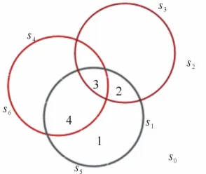
Figure 7. Example of groups of sensors.

To generalize this idea, we can write the equation further. We have si associated to the mother group





* 1

, , , k n

i i i i

G  G G   G 

1

k k

, the order of mother group of s is as the equation below



k *



i i

i

G G

G k  c







*          





Here the integer number  is the count of sub- groups of G*. In addition, c is the repetition.

*

It is clear that G0 0 since the degree of sub-group

1

0 is one and the there is on

G ly one sub-group. Applying this calculation to mother group of sensor







 



* 3 4

1 1, 1 1, 3, 4 , 1, 4, 5 6

1 ,

s G  G G  s s s s s s s , the order





*

1 3 4 2 1 4

G      .

Theorem4: The number of distributed messages sent form si, associated to a mother roup

*

i

G , is g

 

* *

i i i

M Q s G

Proof: The num essages depends on the degree overlapped sensors. The more the degrees of coverage are, the more the areas will be generated. T

get moves

with r

ber of m of

herefore, the more messages will be generated. When a tar

in the range of a senso

 

s1 , it will send notifica- tio

(7)

th_{e sensor will send a notification message to all the} [8] A. Mainwaring, J. Polastre, R. Szewczyk and D. Culler, sensors that cover the same area. *

 

i

Q s is the number of areas inside si which belongs to

*

i

G , and Gi* is

the order of Gi*, then

 

“Wireless Sensor Networks for Habitat Monitoring,” First ACM International Workshop on Wireless Workshop in Wireless Sensor Networks and Applications (WSNA 2002), August 2002. http://dx.doi.org/10.1145/570738.570751 [9] S. C.-H. Huang, S. Y. Chang, H.-C. Wu and P.-J. Wan,

“Analysis and Design of Novel Randomized Broadcast Algorithm for Scalable Wireless Networks in the Inter- ference Channels,” IEEE Transactions on Wireless Com- munications, Vol. 9, No. 7, 2010, pp. 2206-2215.

* *

i i i

M Q s G .

The number of messages of the network in Figure1





  

 



* 1 2 3 4

0 2 3 1 3 4 1

, , ,

, , , , , , , ,

G G G G G

 

, 4 5 6 s s s s s s s s s

 

3. Conclusion

s

gan could

one be

http://dx.doi.org/10.1109/TWC.2010.07.081579

[10] H. H. Zhang and J. C. Hou, “Maximising α-Lifetime for Wireless Sensor Networks,” 2007.

[11] M. Cardei and D. Z. Du, “Improving Wireless Sensor work Lifetime through Power Aware Organization

Net- ,” Wire- We had intr a new method of izing the

sen-so

age and com This new idea be applied in coverage alg in order to control node

target at any oment, and it could used t speed up the routing s as well.

ments

REFERENCES

eless_sensor_network od

m or given

uced unicate. ithms

m algorithm

e

or

less Networks, Vol. 11, No. 3, 2005, pp. 333-340. http://dx.doi.org/10.1007/s11276-005-6615-6 rs of WSN into groups, which would be easy to man-

[12] S. Poduri and G. Sukhatme, “Constrained Coverage for Mobile Sensor Networks,” IEEE International Confer- ence on Robotics and Automation, New Orleans, 26 April- 1 May 2004, pp. 165-172.

and o

one

[13] A. Chen, S. Kumar and T.-H. Lai, “Designing Localized Algorithms for BarrierCoverage,” MOBICOM. ACM, Sep- tember 2007.

[14] X. Bai, Z. Yun, D. Xuan, T

4. Acknowledg

The authors would like to acknowledge The National Natural Science Foundation of China, the National Sci-ence Technology Major Project and the China Scholar-ship Councilfor their supports.

. Lai and W. Jia, “Optimal Pat-

mental Sensor Net- terns for Four-Connectivity and Full Coverage in Wire- less Sensor Networks,” IEEE Transactions on Mobile Computing, 2008.

[15] J. Wu and S. Yang, “Coverage and Connectivity in Sensor Networks with Adjustable Ranges,” International Work- shop on Mobile and Wireless Networking (MWN), Au- gust 2004.

[1] http://en.wikipedia.org/wiki/Wir

[2] C.-Y. Chong and S. P. Kumar, “Sensor Networks: Evolu- tion, Opportunities, and Challenges,” Proceedings of the IEEE, Vol. 91, No. 8, 2003, pp. 1247-1256.

http://dx.doi.org/10.1109/JPROC.2003.814918

[16] M. Cardei, J. Wu, N. Lu and M. O. Pervaiz, “Maximum Network Lifetime with Adjustable Range,” IEEE Interna- tional Conference on Wireless and Mobile Computing, Net- working and Communications (WiMob’05), August 2005. [3] E. Zana di and F. Chiaraluce fficiency

Networks,”

ceedings rence on

So

ft-Computer j,

of M. Bal

Gossip Algorithm for Wirele th

, “E onfe

of the

Pro- [17] M. Cardei, M. T. Thai, Y. Li and W. Wu, “Energy-Effi- _{cient Target Coverage in Wireless Sensor Networks,”} Proceedings of IEEE Infocom, 2005.

[18] M. Cardei and D.-Z. Du, “Improving Wireless Sensor Net- ss Sensor

e 15th International C

ware, Telecommunications and Computer Networks (So COM), Split-Dubrovnik, Croatia, September 2007.

work Lifetime through Power Aware Organization,” Vol. 11, No. 3, 2005, pp. 333-340.

[19] J. K. Hart and K. Martinez, “Environ [4] “Mems and Nanotechnology.” http://www.memsnet.org/

[5] I. F. Akyildiz, W. Su, Y. Sankarasubramaniam and E. Ca-

yirci, “Wireless Sensor Networks: A Survey,” _{works: A Revolution in the Earth System Science?” Earth-} Science Reviews, Vol. 78, 2006, pp. 177-191.

http://dx.doi.org/10.1016/j.earscirev.2006.05.001 Networks, Vol. 38, No. 4, 2002, pp. 393-422.

http://dx.doi.org/10.1016/S1389-1286(01)00302-4 [6] D. Estrin, R. Govindan, J. S. Heidemann and S. Kumar,

“Next Century Challenges: Scalable Coordination in Sensor Networks,” Proceedings of ACM MobiCom’99,

[20] Y. Ma, M. Richards, M. Ghanem, Y. Guo and J. Hassard, “Air Pollution Monitoring and Mining Based on Sensor Grid in London,” Sensors, Vol. 8, No. 6, 2008, p. 3601. http://dx.doi.org/10.3390/s8063601

Washington, August 1999.

[7] J. M. Kahn, R. H. Katz and K. S. J. Pister, “Next Century Challenges: Mobile Networking for “Smart Dust,” Pro- ceedings of ACM MobiCom’99, August 1999.

(8)

Distributed messages of network shown in Figure 1.

si

* 1

G * 

i

Q s  Mi

S0 0 1 1 0

S1 5 10 2 50

S2 1 2 1 2

S3 3 5 2 15

S4 4 8 2 28

S5 3 7 1 21