Multiple classifier architectures and their application to credit risk assessment

Full text

(1)Lancaster University Management School Working Paper 2008/012. Multiple classifier architectures and their application to credit risk assessment. Steven Finlay The Department of Management Science Lancaster University Management School Lancaster LA1 4YX UK. © Steven Finlay All rights reserved. Short sections of text, not to exceed two paragraphs, may be quoted without explicit permission, provided that full acknowledgement is given. The LUMS Working Papers series can be accessed at http://www.lums.lancs.ac.uk/publications/ LUMS home page: http://www.lums.lancs.ac.uk/.

(2) Multiple classifier architectures and their application to credit risk assessment Steven Finlay Department of Management Science, Lancaster University. Abstract. Multiple classifier systems combine several individual classifiers to deliver a final classification decision. An increasingly controversial question is whether such systems can outperform the single best classifier and if so, what form of multiple classifier system yields the greatest benefit. In this paper the performance of several multiple classifier systems are evaluated in terms of their ability to correctly classify consumers as good or bad credit risks. Empirical results suggest that many, but not all, multiple classifier systems deliver significantly better performance than the single best classifier. Overall, bagging and boosting outperform other multi-classifier systems, and a new boosting algorithm, Error Trimmed Boosting, outperforms bagging and AdaBoost by a significant margin. Keywords: OR in Banking, Data Mining, Classifier Combination, Classifier ensembles, Credit scoring. correspondence: steven.finlay@virgin.net. 1.

(3) Introduction Since the early 1990s the majority of consumer lending decisions in the US have been made using automated credit scoring systems (Rosenberg and Gleit, 1994). A similar situation exists in the UK and many other countries. Credit scoring systems are not perfect and every year a significant proportion of consumer debt is not repaid because of the failure of such systems to identify individuals who subsequently default on their loans. The value of outstanding consumer credit (excluding residential mortgage lending) in the US and UK at the end of 2007 was $2.5 trillion and £164 billion respectively (Bank of England, 2008b; The Federal Reserve Board, 2008b). For the same period, annualized write-off rates for credit cards were 4.2 percent and 7.3 percent in the US and UK respectively. For personal loans and other forms of unsecured credit write-off rates were 3.7 percent and 1.9 percent (Bank of England, 2008a; The Federal Reserve Board, 2008a). The losses resulting from defaulting customers is therefore very significant indeed. Consequently, there is considerable interest in improving the ability of credit scoring systems to discriminate between customers on the basis of their future repayment behaviour. Even very small improvements in classification performance can yield considerable financial benefit (Hand and Henley, 1997). Credit scoring is traditionally viewed from a binary classification perspective. Classification or regression methods are used to create a classifier that generates a numerical output (a score) representing the likelihood of an individual being a ‘good’ or ‘bad’ credit risk over a given forecast horizon. Good credit risks are those that repay their debt to the terms of the agreement. Bad credit risks are those that default or display otherwise undesirable behaviour (note that ‘good’ and ‘bad’ are standard terms used within the credit scoring community to describe a two class binary classification problem of this type and these terms are used from now on). Some methods applied in credit scoring produce probabilistic estimates of class membership, but some do not, and what is of primary importance is the relative ranking of model scores (Thomas et al., 2001a). Lending decisions are made on the basis of the properties of the ranked score distribution, with a cut-off being defined that meets the business objectives of the user. As long as an observation is correctly classified, then the margin by which an observation passes or fails the cut-off is largely irrelevant (Hand, 2005). In some cases the cut-off may be based on a likelihood measure, such as the point in the score distribution where the good:bad odds ratio exceed 10:1. In other cases the cut-off is chosen to yield a fixed proportion of 2.

(4) accepted applications. For example, a provider of retail credit may agree to provide credit to customers of a furniture retailer where there is a contractual obligation to accept at least 90% of all credit applications. In practice, measures of group separation, such as the GINI coefficient and the KS statistic, are also popular, but such measures are only of interest in two situations. First, when the cut-off decision(s) are unknown at the time when the model is developed – a situation facing the developers of generic scoring models that are used by many different lenders. Second, where multiple cut-offs are required so that different terms can be applied to individuals on the basis of their risk – a practice referred to as “Pricing for risk.” Credit scoring was one of the first and most successful applications of data mining. What differentiates credit scoring from other data mining applications are the objectives of the financial institutions that employ it, the nature of the data sets employed and the business, social, ethical and legal issues that constrain its use within decision making processes. The most popular methodology applied to credit scoring is logistic regression (Crook et al., 2007). Other methods such linear regression/discriminant analysis (Durand, 1941; Myers and Forgy, 1963) and decision trees (Boyle et al., 1992) are also popular. This is principally because they are easy to develop, yield acceptable levels of performance and the structures of the resulting classifiers are easily explicable in support of legislative and operational requirements. In recent years, there has been increasing use of neural networks (Desai et al., 1996; West, 2000) but these tend to be restricted to fraud detection and other back-end credit scoring processes where a lower level of explicability is required (Hand, 2001). Within the academic community there has been a growing body of literature into the application of many other methodologies. Some are statistical approaches such as survival analysis (Narain, 1992; Stepanova and Thomas, 2001), graphical models (Sewart, 1997), K-Nearest Neighbour (Henley and Hand, 1996), Markov chains (Thomas et al., 2001b) and quantile regression (Whittaker et al., 2005). Others are from the machine learning/data mining domain. Examples include genetic algorithms (Desai et al., 1997; Finlay, 2005) and support vector machines (Baesens et al., 2003; Huysmans et al., 2005). Empirical evidence from a number of studies has shown little support for any one classification or regression methodology consistently outperforming any other in terms of misclassification rates/cost or measures of group separation (Baesens et al., 2003; Boyle et al., 1992; Desai et al., 1996; Henley, 1995; West, 2000). Looking at the cumulative findings from across these studies there is some evidence that non-linear approaches such 3.

(5) as neural networks and support vector machines do, on average, outperform other methods (Crook et al., 2007), but only by a very small margin, and there is no consensus as to which methodology a model developer should adopt for a given problem. Given this uncertainly, it is not unusual for a practitioner to construct several different classifiers, using different techniques, and then choose the one that yields the best results for their specific problem. It does not necessarily follow that the best single classifier dominates all others over all regions of the problem domain, and error rates can often be reduced by combining the output of several classifiers (Kittler, 1998). As noted by Zhu et al. (2001), the general research into classifier combination (also referred to as classifier fusion or classifier ensembles) is rich, with a considerable number of papers published in the decade prior to their paper. However, within the credit scoring community the number of papers relating to classifier combination is sparse and few report empirical findings on data sets that can be said to be representative of those found in industry. Instead, most are based on “Toy” data sets, that are only a fraction of the size and/or dimensionality of the data sets employed by major financial institutions in first world credit markets, such as those in the US and UK (Finlay, 2006). In addition, previous studies have had a narrow focus. Standard practice has been to compare a single benchmark classifier with a narrow set of multiple classifier systems, often employing just one method of classifier construction. There has been little effort to compare and contrast the wide range of multiple classifier systems available in conjunction with the different mechanisms by which classifiers can be constructed. The remainder of the paper is in two parts. In the first part I describe the types of multiple classifier architectures that can be employed, followed by a review of the literature relating to their application to credit scoring problems. In the second part of the paper a variety of multiple classifier systems are evaluated in terms of their ability to correctly classify good and bad credit risks. For this purpose two comprehensive real world data sets are employed that have been supplied by industry sources. It would be impossible to cover all possible variants of multiple classifier systems in a single paper. Therefore, the emphasis has been to report on a representative sample of well known examples, for which empirical evidence exists that they can yield improved performance over a single classifier. In. 4.

(6) addition, a new multi-classifier algorithm – Error Trimmed Boosting (or ET Boost for short) is presented and its performance compared to the other systems under discussion.. Multiple Classifier System Architectures Multiple classifier system can be classified into one of three architectural types. The first, and probably the most popular, are static parallel (SP) systems where two or more classifiers are developed independently in parallel (Zhu et al., 2001). The outputs from each Ct (t=1...T) classifier are then combined to deliver a final classification decision w =. φ (C1 ...C t =T ) , where w is selected from the set of possible class labels. A large number of combination functions are available. These include simple majority vote, weighted majority vote, the product or sum of model outputs, the min rule, the max rule and Bayesian methods. However, in practice most combination strategies are reported to yield very similar levels of performance (Kittler, 1998). Consequently, simple majority vote or weighted majority vote are often favoured due to their simplicity of application and their applicability to situations where the raw outputs from each classifier may not all be interpretable in the same way. Another option is for the outputs from each classifier to be used as inputs to a second stage classifier that delivers the final classification decision (Kuncheva et al., 2001). Some SP approaches use identical representations of the data, but apply different methods of construction to produce each classifier such as neural networks, linear regression and CART. Classifier outputs are then combined to produce the final classification decision. Other SP approaches utilize a single method for classifier construction, but use different representations of the data to produce each classifier. Two such examples are cross validation and bagging. With cross-validation data is segmented into k folds. k models are then constructed with a different fold excluded for each model. With bagging (bootstrap aggregating) (Breiman, 1996), classifiers are constructed from different sub-sets of the data randomly sampled with replacement. Breiman developed bagging further with random forests (Breiman, 2001), where further random elements are entered into the procedure, for example randomly selecting subsets of variables or randomly selecting the order in which good predictors are applied.. 5.

(7) The second type of architectures are multi-stage (MS) ones. Classifiers are constructed iteratively. At each iteration the parameter estimation process is dependent upon the classification properties of the classifier(s) from previous stages. Some MS approaches generate models that are applied in parallel using the same type of combination rules used for SP methods. For example, most forms of boosting (Schapire, 1990) generate a set of weak classifiers that are combined to create a stronger one. This is achieved by employing a re-sampling/reweighting strategy at each stage, based on a probability distribution or heuristic rule, derived from the misclassification properties of the classifier(s) from the previous stage(s). As the boosting algorithm progresses increasing focus is placed on harder to classify/more borderline cases. The boosting algorithm terminates after a given number of iterations have occurred or some other stopping criteria is met. Classifier output from each stage is then combined to make the final classification decision. The most well known boosting algorithm is arguably AdaBoost (Freund and Schapire, 1997) and many variants have subsequently appeared such as Arc-x4 (Breiman, 1998), BrownBoost (Freund, 2001) and LogitBoost (Friedman et al., 2000). Other MS methods produce a separate classifier at each stage and then classify a proportion of observations at that stage. The next stage classifier is then developed and applied to the remaining, unclassified, population. A variation on this theme is to make the final classification decision for all observations using a single classifier from one stage with all other classifiers being discarded (Myers and Forgy, 1963). The classifier produced from such an approach may in theory be sub-optimal, but improved classification can result because “outliers” at the extreme ends of the class distribution are excluded, allowing the decision surface to be obtain a better fit to more marginal cases while still correctly classifying the excluded cases. This approach also has a practical advantage in that it results in a single classifier. This makes it more attractive in operational environments than MS methods such as boosting because it is much simpler to implement and monitor a single classifier than multiple classifiers with serial dependencies. The third type of multiple classifier architecture is Dynamic Classifier Selection (DCS). Different classifiers are developed or applied to different regions within the problem domain. While one classifier may be shown to outperform all others based on global measures of performance, it may not dominate all other classifiers entirely. Weaker competitors will sometimes outperform the overall best across some regions (Kittler, 6.

(8) 1997). DCS problems are normally approached from a global (DCS-GA) or local accuracy (DCS-LA) perspective (Kuncheva, 2002). With a DCS-GA approach classifiers are constructed using all observations within the development sample. Classifier performance is then assessed over each region of interest and the best one chosen for each region. One limitation of the DCS-GA approach is that while different classifiers may be shown to perform better within certain regions than others, there is no guarantee that any given classifier is optimal within any given sub-region, and that better classification might result if a separate classifier is developed specifically for that region. With a DCS-LA approach, regions of interest are determined first, then separate classifiers developed for each region. An issue in this case is one of sample size. While it is relatively easy to construct a classifier and confirm that it is robust and not over-fitting, if the sample size upon which it has been developed is small then the locally constructed classifier may be inefficient and not perform as well as a classifier developed on a larger more general population. Consequently, there is a trade-off between the robustness of classifiers developed using large samples with the ability to identify features within sparsely populated areas of the problem domain, and the accuracy of local classifiers. This logically leads to the conclusion that for DCS-LA approaches one benchmark against which performance should be measured are the results obtained from applying a DCS-GA approach and vice versa. With DCS-GA and DCS-LA approaches an important issue is identifying the best regions to develop or apply classifiers to. In some situations regions are defined using purely mechanical means. For example, the method described by Kuncheva (2002) is to apply a clustering algorithm, such as K-Nearest Neighbour. An improvement over simple clustering was reported by Liu and Yuan (2001) who applied a two-stage approach containing both global and local components. First they constructed classifiers across the entire problem domain, then applied K-NN clustering to generate two sets of clusters containing observations that had been correctly or incorrectly classified by each classifier. Second stage classifiers were then constructed for each cluster and used to make the final classification decision. In many applied situations segmentation decisions are constrained by practical considerations that may limit the usefulness of purely mechanical methods such as clustering. Segmentation decisions will be overwhelmingly driven by expert knowledge, business considerations, legal or other environmental constraints. For example, Toygar and Acan (2004) successfully applied a DCS-LA approach to face recognition problems. They segmented faces into regions by simply dividing the images in their data 7.

(9) set into a set of equally sized horizontally strips so that specific features such as nose, eyes, mouth etc. fell into each strip. The rationale for choosing this segmentation was primarily expert opinion about the regions which are important in face recognition problems, and trial and error. The approaches exemplified by Toygar and Acan (2004) and Liu and Yuan (2001) represent two ends of a spectrum. At one end segmentation is entirely determined by mechanical segmentation rules, and at the other, segmentation decisions are made subjectively by experts within a field. Consumer credit is an area that falls somewhere in the middle of this spectrum. As noted by Thomas et al. (2002). Mechanical means of segmenting a problem domain may be employed, such as applying the splitting rules associated with the construction of decision trees. However, segmentation is often driven by political decisions, the availability of data, product segmentation (e.g. cards and loans) or other business rules.. Applications of Multiple Classifier System for Consumer Credit Risk Assessment A common strategy applied in credit scoring is to develop sub-population models for different regions of the problem domain (Banasik et al., 1996). Sub-population modelling is an example of a DCS-LA architecture, and most classifier combination strategies reported in the credit scoring literature adopt a DCS-LA approach, even if they are not described as such. One reason why a DCS-LA strategy is attractive is that each model is developed and applied independently to a different region of the problem domain. Therefore, each credit application is only scored by a single model. From an implementation perspective this is attractive because it simplifies performance monitoring, facilitates the redevelopment of models on a piecemeal basis and generates scorecards that are more readily explicable to the general public in support of legislative requirements. This is regardless of the method used to generate the segments upon which the subpopulation models are constructed, and therefore offers a methodology whereby techniques that do not generate a simple (linear) parameter structure, such as clustering, neural networks or support vector machines, can be combined with methods that do. For example, the output from a complex (difficult to interpret) neural network model could be used to define segments upon which simple linear scoring models are then constructed. If probabilistic estimates of class membership are required, then as long as the final models generate probabilistic estimates, then it is irrelevant whether the segmentation strategy does so or not. Not all of these properties can be said to be universally true of static parallel or multi-stage classifier systems. 8.

(10) Empirical analysis of credit data would lend some, but not overwhelming, support for DCS-LA methodologies providing improved classification performance over a single global classifier. Chandler and Ewert (1976) compared a single model using gender as a dummy variable with two models developed for males and female credit applicants respectively. One of their findings was that the two separate models used in combination led to a lower rate of rejected female applicants than the single model. Banasik et al. (1996) explored this further, examining the performance of a single credit scoring model against models constructed on twelve different segmentations such as married/not married, retired/not retired and so on. They concluded that using sub-population models sometimes led to better solutions, but this was not always the case. Another strategy along these lines was investigated by Hand et al. (2005) who considered binary segmentation using an “optimal partition” strategy based on maximising the product of two likelihood functions calculated from observations in each of the two potential segments. They observed small but significant improvements in classification performance. In another study, a preliminary forecasting model was constructed to estimate usage on a revolving credit product. The population was then segmented into two parts on the basis of whether the estimated usage was high or low (Banasik et al., 2001). The conclusion was that the performance of the two sub-population models was superior to that of a single model constructed across the entire population, but that the improvement was marginal. The limited research undertaken into the application of other types of classifier combination to credit scoring problems has arguably yielded better results than DCS-LA approaches. Myers and Forgy (1963) adopted a multi-stage approach in which they utilised a two stage discriminant analysis model. The second stage model was constructed using the worst performing 86% of the original development sample. They reported that the resulting second stage model identified 70% more bad cases than the first stage model on its own for their chosen cut-off strategy. This idea has some parallels with boosting strategies that apply weight trimming rules to exclude observations that have insignificant weights because they are classified correctly with a high degree of confidence (Friedman et al., 2000). Yachen (2002) reported up to 3% improvement in GINI coefficient when applying a logistic model, followed by a neural network. Zhu et al. (2001) reported improvements of 9.

(11) between 0.5% and 1.3% when using a logistic function to combine two scores, each constructed using different sets of features but with the same target variable. Zhu et al. (2002) applied a SP approach to combine classifiers constructed using discriminant analysis, logistic regression and neural networks using a Bayesian combination rule. The results showed increasing performance as the number of classifiers increased, yielding similar, but not superior, performance to the single best classifier, which may have been a result of over fitting given the markedly better performance seen on the development data set compared to the validation set. West Dellana et al. (2005) compared ensembles of neural networks constructed using cross-validation, bagging and boosting (AdaBoost) against the single best network for three different data sets. They found that both bagging and cross validation yielded statistically significant reductions in classification error of 2.5% and 1.9% respectively, averaged across the three data sets. However, boosting was reported to yield significantly worse error rates than a single classifier, which was attributed to outliers, noise and mislabelled learning examples. Although these studies have utilized different data sets and different methodologies, two interesting features stand out. The first is that the greatest uplift in performance is reported by Myers and Forgy (1963) with their simple 2-stage MS strategy, utilizing the second stage model to make the final classification decision. They effectively used the first stage model to identify “outliers” at the extreme end of the score distribution, allowing the classification model to be constructed on marginal cases around the desired cut-off – somewhat similar in principle to the idea underpinning support vector machines. The second is that there has been relatively little research effort to compare and contrast different multiple classifier systems in conjunction with different classification methodologies within the credit scoring arena (and to the best of my knowledge classification problems in general). Only in the study by West Dellana et al. (2005) was more than a single combination strategy given consideration, and in this case only one type of classifier (neural networks) was considered.. Experimental Design Four base methods of classifier construction were considered: logistic regression (LR), linear discriminant analysis (LDA), classification and regression trees (CART) and artificial neural networks (NN). LR, LDA, CART and NN were chosen for a number of reasons. First, each utilizes a different form of parameter estimation/learning. Second, 10.

(12) between them they generates three different model forms; linear models, trees and networks. Third, all are practically applicable within operational consumer lending environments, with known examples of their application within the financial services industry. To begin, single classifiers were constructed using each method. These were used to provide benchmarks against which various multiple classifier systems were assessed. For CART models binary splitting rules were employed based on maximum entropy. The part of the data set allocated to model development was further segmented 80/20 train/test. The tree was grown using the 80 percent allocated for training. Pruning was then applied based on minimized sum of squared error, calculated using the 20 percent validation sample, as advocated by Quinlan (1992). For neural network models a MLP architecture was adopted with a single hidden layer, and as for CART, development data was segmented 80/20 train/test. For each data set the network structure and training criteria were determined a priori based on the results from a number of preliminary experiments (the resulting network structure was then used for all experiments involving that data set; that is, all networks trained using a given data set had the same number of units in the hidden layer, the same activation function, training algorithm and so on.) Preliminary experiments were performed using a randomly selected 50 percent of observations split 80/20 train/test (50 percent was used to correspond with the size of the folds used in model development – as described below). N-1 models were created using 2,3,…,N hidden units, where N was equal to the number of inputs. The performance of each model was then evaluated on the test set. A 5-fold strategy was applied, with a different fold acting as the test set each time. An average of the number of hidden units in the best model for each of the five folds was taken, rounded up to the nearest whole number, and this was the number of hidden units used for all subsequent experiments. Given the size of the data sets employed and the number of independent variables it was considered unlikely that over-fitting would be an issue for any reasonable number of hidden units. Given the number of experiments performed, a relatively fast training algorithm was necessary to allow experiments to be completed in realistic time. For this reason network training utilized the quasi-Newton algorithm with a maximum of 200 training epochs. Five types of static parallel multiple classifier system were explored. The first static parallel system combined the output of the baseline classifiers to produce a final 11.

(13) classification decision using a simple majority vote. All possible combinations of three classifiers (from four) were explored. These are designated SP1-NOCART, SP1-NOLR, SP1-NOLDA and SP1-NONN respectively, to indicate which classifier score was excluded. The second static parallel system, SP2, applied stepwise logistic regression to generate a weighted function of the four baseline classifier scores. SP3 used a neural network with a single hidden layer to produce a final score. The four baseline scores acted as inputs, and four units were included in the hidden layer. SP4-LR applied cross validation. Stratified random sampling was applied to allocate observations to one of 50 equally sized folds. 50 classifiers were then constructed using 49 of the folds, with a different fold excluded from each model. A final classification decision was then made using simple majority vote. In the case of tied votes the final classification decision was chosen at random. SP4-LDA, SP4-CART and SP4-NN applied cross validation again, but this time for LDA, CART and NN respectively. SP5-LR applied bagging with logistic regression, using 50 independently drawn samples with replacement. The final classification decision was made using simple majority vote. SP5-LDA, SP5-CART and SP5-NN applied an identical bagging algorithm using LDA, CART and NN respectively. Three multi-stage classifier systems were investigated. The first multi-stage classifier system, MS1-LR, is the Discrete AdaBoost algorithm as described in Figure 1, applied to logistic regression. 1. Initialise t=0 2. Initialise a probability distribution D0(i)= 1/ n0 for all i ∈ (1… n0) 3. DO While t<T 4. 5.. Construct classifier Ct from M0 using weights Dt n0. Calculate weighted error as: Et = ∑ Dt (i ) C t (xi ) − y i i =1. 6.. IF Et ≤ 0 OR Et ≥ 0.5 then STOP. 7.. ⎛ 1 − Et Calculate α t = 0.5 ln⎜⎜ ⎝ Et. ⎞ ⎟⎟ ⎠. 8.. Create distribution Dt +1 (i ) =. Dt (i ) exp(− α t y i C t ( xi )) Zt. 9.. t=t+1. 10. END While loop. 12.

(14) T −1. 11. Assign final classification decision as C*= ∑ (α t C t ( x )) t =0. Figure 1. The Discrete AdaBoost Algorithm In Figure 1, The training set M0 is defined as containing n0 observations (x1, y1)...(xn0,yn0) with class labels y ∈ (-1,+1). At each iteration of AdaBoost a classifier is constructed using the weighted population (Step 4). A sum of errors measure (Et in Step 5) is then calculated and applied to adjust the weighting assigned to each observation (Step 8). The result is that the weight assigned to correctly classified cases is diminished, while the weight for incorrectly classified cases is increased. Zt in step 8 is a normalizing constant, chosen such that the sum of weights at each iteration are equal to one. The final classification decision is then made using a weighted majority vote (Step 11). The choice of T is problem specific, but values ranging from 25 to 100 are widely quoted in the literature. For the purpose of this study T was set to 50, following preliminary testing that indicated no performance improvements results from having more iterations than this. The second multi-stage classifier system, MS2-LR, is a new boosting algorithm designated Error Trimmed Boosting (or ET Boost for short). As described in Figure 2, ET Boost applies a trimming strategy that successively removes well classified cases from the training set. 1.. Initialize t=0. 2.. DO while t<T. 3.. Construct classifier Ct from Mt. 4.. eti=ƒ(yi, Ct(xi)) , xi ∈ M0, i=1.. n0. 5.. sort elements of M0 in ascending order of eti. 6.. nt+1= INT(nt*λ). 7.. Create set Mt+1 containing first nt+1 elements of M0. 8.. t=t+1. 9.. END while. 10.. Assign final classification decision as C* = φ (C 0 ...CT −1 ). Figure 2. Error Trimmed Boosting (ET Boost) algorithm. 13.

(15) With ET Boost, at the tth iteration the error, eti, is calculated for all n0 observations using classifier Ct (Step 4). Then, INT(nt* λ), (0< λ<1) observations with the largest error are selected for construction of the t+1th classifier (Steps 5-7). λ is a control parameter that determines the rate at which the size of the development sample decreases between subsequent iterations. Note that a key feature of ET Boost is that at each iteration all observations are reconsidered for inclusion in classifier construction. There is no weighting of observations. Thus observations excluded from classifier construction in one iteration may be included in the next iteration if the relative error of an observation increases between subsequent iterations. ET Boost is a very simple, yet flexible, boosting algorithm because it can cater for many different error functions and many different combination functions (step 10). It can also be applied to any type of classifier/regression methodology, regardless of whether or not they generate likelihood estimates, and can therefore be applied to problems with multi-category or continuous outcomes. For the purpose of this study, the error function is chosen to be absolute error: |yi-Ct(xi)|. Simple majority vote is applied as the combination function to put ET Boost on equal footing with bagging and cross validation. Exploratory analysis showed ET Boost to yield good performance for a wide range of values of λ and T. These parameters were therefore chosen on a somewhat arbitrary basis to be 0.975 and 50 respectively. MS3-LR utilizes the individual classifiers developed for MS2-LR. In each case the classification decision is made using the single best classifier from the set of T available classifiers. MS3 can be considered a generalization of the 2-stage strategy utilized by Myers and Forgy (1963). MS1-LDA,…,MS3-LDA, MS1-CART,...,MS3-CART and MS1NN,…,MS3-NN were generated using LDA, CART and NN respectively Two local accuracy dynamic classification systems where explored. For the first, DCSLA1-L-LR, the ranked scores from the baseline logistic regression model were used to segment the population into L segments, with segment boundaries chosen to maximize the entropy across the L segments. LR was then applied to generate a separate model for each segment. The process was then repeated for LDA, CART and NN. For the purposes of this exercise values of L=2 and L=4 were considered. For DCS-LA2-K-LR a clustering algorithm was applied using nearest centroid sorting to create K clusters, with values of. K= 2 and 4 considered. Logistic regression was then applied to each of the resulting clusters. The process was repeated with LDA, CART and NN. A single DCS-GA strategy 14.

(16) was considered, DCS-GA-K. For each of the K clusters defined for DCS-LA2-K, the performance of the four baseline classifiers was measured and the best one chosen for K=2 and 4 to generate solutions DCS-GA-2 and DCS-GA-4 respectively.. Evaluating Performance The performance of each classifier system was assessed on the misclassification rate for the cut-off score, S, where S was the score for which 100* Nb/(Ng+Nb) percent of the population scores S or below. Ng and Nb are the numbers of goods and bads respectively. Therefore, using this cut-off strategy, a perfect classifier would correctly assign all goods scores greater than S and all bads scores less than or equal to S. For dynamic classifier systems that consider several independent sub-regions, separate values of the cut-off score,. S, were defined for each region. Performance metrics were calculated using kj-cross validation which is a variant on standard k-fold cross validation. The population is first segmented into k equally sized folds, F1,…Fk using stratified random sampling. A model is then constructed with fold Fi ,i ∈ (1,…,k) assigned as the validation fold. The validation fold Fi is then segmented into j sub-folds for which performance metrics are calculated. The process is repeated, k times, generating a population of k*j performance measures. The performance of two classifier systems can then be compared using a paired t-test. kj-cross validation is computationally cheap compared to many other validation methods. It is suitable for situations where large data sets are available and experiments are concerned with the comparative performance of competing classification techniques, rather than obtaining the best performance across the entire data set upon which classifiers are being constructed. Another desirable of feature of. kj-cross validation is that for the special case where k=2, each model is constructed and validated using independent data sets. This overcomes the problem of non-independence of the training data associated with standard k-fold validation (k>2) which can lead to inflated values of test statistics when applying paired t-tests (Dietterich, 1998). For the purpose of this study k=2, j=25.. Empirical Data Two real world data sets were available. Data set A was supplied by the Experian credit reference agency in the UK. It contained details of retail credit applications made to several mainstream lending institutions between April and June 2002. It can therefore be 15.

(17) taken as providing a representative picture of the UK population of retail credit applications. 12 month performance data was attached and this was used to generate a +1,1 target variable (Good=1, bad=-1). Those <= 1 month in arrears, and no history of seriously delinquency within the last 6 months (3+ months in arrears) were classified as good. Those currently 3+ more months in arrears, or 3+ months in arrears any time within the last 6 months were classified as bad. All other cases where classified as “indeterminate” and excluded. This definition of good/bad is consistent with those applied by practitioners, based on bads being three or more cycles delinquent and goods as up-todate or no more than one cycle delinquent (Hand and Henley, 1997; Lewis, 1992; McNab and Wynn, 2003). The final data set contained 88,789 observations of which 75,528 cases were classified as good and 13,261 as bad. 39 independent variables were available. These included applicant provided information such as age, residential status and income, as well as a common credit reference data such as number, value and time since most recent delinquency, account performance history, number of recent credit searches, time on electoral roll and Experian’s MOSAIC postcode level classifier. Data set B was a large behavioural scoring data set provided by a supplier of revolving credit. Performance data was attached 12 months after the sample date. Goods were defined as <=1 month in arrears, bads as 3+ months in arrears. After removing exclusions, such as indeterminates, dormant accounts and those already classified as bad, the data set contained 120,508 goods and 18,098 bads. 54 independent variables were available, examples of which were current and historic statement balance, arrears status, payments and various ratio’s of these variables over 3,6 and 12 months. Data pre-processing was performed using the weights of evidence transformation. This is a standard pre-processing technique applied to credit scoring problems (Crook et al., 2007; Finlay, 2008; Hand and Henley, 1997; Siddiqi, 2005). Continuous variables such as income were binned into a number of discrete categories, and the weight of evidence in ⎛ (g G ) ⎞ ⎟⎟ , where G and B are the number of goods and bads in each bin calculated as LN ⎜⎜ i ( ) b B ⎠ ⎝ i. the population, and gi and bi are the number of goods and bads within the ith bin. The weight of evidence was then substituted for the true attribute value. For categorical variables each category was allocated to a separate bin. In cases where a category. 16.

(18) contained relatively few observations coarse classing, as described by Thomas et al. (2002) was applied and the category combined with another. Note that when applying methods that perturb the data, such as bagging and boosting, the weights of evidence must be recalculated each time the data is modified to take into account the changing proportion of goods and bads within each bin. After pre-processing, a preliminary variable selection exercise was undertaken. A stepwise logistic regression procedure was applied to the full population with a 5% significance level applied for model entry/exit. The data was segmented into 5 folds, with a model built using the first four folds. The process was repeated five times with a different fold excluded on each occasion. Any variable appearing in any of the 5 models was retained for the main modelling exercise. After preprocessing and variable selection, 29 of original 39 variables were available for model construction for data set A. For data set B 37 variables were selected.. Results and Findings Table 1 shows the percent of misclassified cases, and the improvement over the baseline for each classifier system.. 17.

(19) Data set A Classifier system. Data set B. % Misclassified. % Absolute improvement over baseline. % Relative improvement over baseline. % Misclassified. % Absolute improvement over baseline. % Relative improvement over baseline. 13.07% 13.25% 14.41% 13.17%. 0.00% -1.43% -10.27% -0.81%. N/A N/A N/A N/A. 14.96% 15.24% 15.65% 14.89%. -0.53% -2.36% -5.14% 0.00%. N/A N/A N/A N/A. 13.05% 12.94% 12.67% 13.06% 12.49% 12.22% 13.07% 13.25% 13.57% 13.09% 13.05% 13.23% 12.26% 13.03%. 0.12% 0.97% 3.03% 0.08% 4.41% 6.45% 0.00% -1.37% -3.84% -0.19% 0.16% -1.21% 6.17% 0.30%. N/A N/A N/A N/A N/A N/A 0.00% 0.06% 5.83% 0.61% 0.16% 0.22% 14.91% 1.10%. 14.77% 14.79% 14.54% 14.93% 14.33% 14.27% 14.96% 15.24% 14.87% 14.88% 14.95% 15.25% 13.93% 14.82%. 0.77% 0.62% 2.32% -0.30% 3.76% 4.16% -0.48% -2.35% 0.07% 0.03% -0.43% -2.44% 6.44% 0.44%. N/A N/A N/A N/A N/A N/A 0.05% 0.01% 4.96% 0.03% 0.10% -0.08% 11.02% 0.44%. 13.04% 13.07% 13.88% 13.02% 12.34% 12.65% 11.92% 11.64% 12.97% 13.07% 14.36% 13.05%. 0.18% 0.02% -6.21% 0.36% 5.60% 3.18% 8.75% 10.91% 0.74% 0.00% -9.91% 0.15%. 0.18% 1.43% 3.69% 1.16% 5.60% 4.54% 17.25% 11.62% 0.74% 1.41% 0.33% 0.96%. 14.96% 14.95% 15.31% 14.78% 13.37% 13.79% 13.06% 12.92% 14.89% 15.03% 15.65% 14.76%. -0.50% -0.46% -2.86% 0.71% 10.16% 7.34% 12.27% 13.19% -0.01% -0.99% -5.14% 0.86%. 0.03% 1.86% 2.17% 0.71% 10.63% 9.48% 16.56% 13.19% 0.51% 1.33% 0.00% 0.86%. 15.07% 16.16% 14.82% 15.64% 15.97% 16.33% 15.01% 16.02% 13.67% 14.05% 13.80% 14.08% 15.29% 15.92% 13.71% 14.18% 13.37% 14.02%. -15.32% -23.69% -13.43% -19.69% -22.20% -24.96% -14.84% -22.56% -4.60% -7.55% -5.59% -7.74% -17.03% -21.81% -4.95% -8.52% -2.34% -7.26%. -15.32% -23.69% -11.83% -18.00% -10.82% -13.32% -13.92% -21.58% -4.60% -7.55% -4.10% -6.22% -6.13% -10.46% -4.10% -7.64% N/A N/A. 15.93% 16.90% 15.93% 16.90% 18.06% 18.22% 16.06% 17.43% 15.28% 15.61% 15.49% 15.67% 16.71% 17.16% 15.33% 15.66% 15.65% 15.63%. -7.03% -13.55% -7.03% -13.55% -21.31% -22.41% -7.86% -17.09% -2.63% -4.84% -4.07% -5.28% -12.24% -15.30% -2.98% -5.18% -5.14% -5.01%. -6.47% -12.96% -4.56% -10.94% -15.38% -16.42% -7.86% -17.09% -2.09% -4.29% -1.68% -2.85% -6.75% -9.66% -2.98% -5.18% N/A N/A. Baseline models LR LDA CART NN. Static parallel SP1-NOLR (simple majority vote ) SP1-NOLDA (simple majority vote ) SP1-NOCART (simple majority vote ) SP1-NONN (simple majority vote ) SP2 (Logistic regression combination) SP3 (Neural network combination) SP4-LR (cross validation) SP4-LDA (cross validation) SP4-CART (cross validation) SP4-NN (cross validation) SP5-LR (bagging) SP5-LDA (bagging) SP5-CART (bagging) SP5-NN (bagging). Multi-stage MS1-LR (adaboost) MS1-LDA (adaboost) MS1-CART (adaboost) MS1-NN (adaboost) MS2-LR (ET Boost) MS2-LDA (ET Boost) MS2-CART (ET Boost) MS2-NN (ET Boost) MS4-LR (ET Boost, best single model) MS4-LDA (ET Boost, best single model) MS4-CART (ET Boost, best single model) MS4-NN (ET Boost, best single model). Dynamic classifier selection DCS-LA1-2-LR (score based segments) DCS-LA1-4-LR (score based segments) DCS-LA1-2-LDA (score based segments) DCS-LA1-4-LDA (score based segments) DCS-LA1-2-CART (score based segments) DCS-LA1-4-CART (score based segments) DCS-LA1-2-NN (score based segments) DCS-LA1-4-NN (score based segments) DCS-LA2-2-LR (cluster based segments) DCS-LA2-4-LR (cluster based segments) DCS-LA2-2-LDA (cluster based segments) DCS-LA2-4-LDA (cluster based segments) DCS-LA2-2-CART (cluster based segments) DCS-LA2-4-CART (cluster based segments) DCS-LA2-2-NN (cluster based segments) DCS-LA2-4-NN (cluster based segments) DCS-GA-2 DCS-GA-4. Table 1. Performance of competing classifier systems. 18.

(20) In Table 1 the performance of the single best baseline model is taken as the reference point in the “Absolute improvement” columns. Figures refer to incremental improvement. Therefore, if system X misclassifies 20% of cases and system Y misclassifies 19% of cases the improvement of Y over X is calculated as 5%. The “Relative improvement” columns are for classifier systems that utilize only a single form of classifier. The figures in this column refer to the improvement over the base line classifier of that type. For example, for SP4-NN (cross validation with neural networks) for data set A the improvement over the baseline neural network model is 0.61%. Shaded cells indicate that performance is superior to the baseline model at a 99% level of significance. Let us begin by examining the performance of the baseline classifiers. LR and NN are the best for data sets A and B respectively, and in each case the differences between LR and NN are statistically significant, but small in percentage terms. In both cases the performance of CART is considerably worse than other methods. This is despite a number of preliminary experiments that looked at different pruning/data pre-processing strategies. These preliminary experiments suggested that for credit scoring data sets, using discretorized (weights of evidence) data gave superior performance than using continuous variables in their raw form or dummy variables. This is a conclusion supported by Baesens et al. (2003) who also found that using discretorized data yield better results CART. Overall, the results for the baseline classifiers are not particularly surprising and are compatible with previous empirical studies of classifier performance for credit scoring data sets. All of the static parallel systems show some potential to significantly outperform the baseline. However, cross validation and Bagging are weakest, with only ensembles using CART showing any major improvement (SP4-CART and SP5-CART). Simple majority vote of the base line classifiers is also poor, showing at best modest improvements, with the exception of SP1-NOCART. The two best performing static parallel systems are SP3 (neural network combination of the base line classifiers), and SP5-CART (Bagging with decision trees). For data set A SP3 is best, closely followed by SP5-CART, with improvements of 6.45% and 6.15% respectively. For data set B the situation is reversed. SP5-CART provides 6.44% improvement compared to 4.15% for SP3. The linear weighting function (SP2), derived using stepwise logistic regression, also performs well, 19.

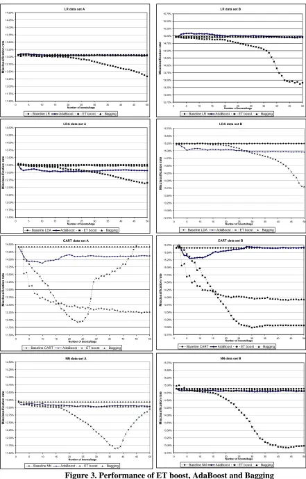
(21) providing a respectable 4.41% and 3.76% improvement over the single best classifier for data sets A and B respectively. Multi-stage systems also provide statistically significant benefits over the baseline models. The clear winner in this category (and best across all categories and both data sets) is ET boost, which provides large and significant improvements over the baseline and other multiple classifier systems for all methods considered, with best performance when applied to neural networks. The performance of ET boost, compared with bagging and AdaBoost is shown in Figure 3.. 20.

(22) LR data set B 15.75%. 14.25%. 15.50%. 14.00%. 15.25%. 13.75%. 15.00%. 13.50%. Misclassification rate. Misclassification rate. LR data set A 14.50%. 13.25% 13.00% 12.75% 12.50%. 14.75% 14.50% 14.25% 14.00% 13.75%. 12.25%. 13.50%. 12.00%. 13.25%. 11.75%. 13.00%. 11.50%. 12.75% 0. 5. 10. 15. Baseline LR. 20 25 30 Number of boosts/bags. AdaBoost. ET boost. 35. 40. 45. 50. 0. 5. Bagging. 10. 15. Baseline LR. 15.75%. 14.25%. 15.50%. 14.00%. 15.25%. 13.75%. 15.00%. 13.50% 13.25% 13.00% 12.75% 12.50%. 35. 40. 45. 50. Bagging. 14.75% 14.50% 14.25% 14.00% 13.75%. 12.25%. 13.50%. 12.00%. 13.25%. 11.75%. 13.00%. 11.50%. 12.75%. 0. 5. 10. 15. Baseline LDA. 20 25 30 Number of boosts/bags. AdaBoost. ET boost. 35. 40. 45. 50. 0. 5. 10. 15. Baseline LDA. Bagging. 20 25 30 Number of boosts/bags. AdaBoost. ET boost. 35. 40. 45. 50. 40. 45. 50. 40. 45. 50. Bagging. CART data set B. CART data set A 14.50%. 15.75%. 14.25%. 15.50%. 14.00%. 15.25%. 13.75%. 15.00%. Misclassification rate. Misclassification rate. ET boost. LDA data set B. 14.50%. Misclassification rate. Misclassification rate. LDA data set A. 13.50% 13.25% 13.00% 12.75% 12.50%. 14.75% 14.50% 14.25% 14.00% 13.75%. 12.25%. 13.50%. 12.00%. 13.25%. 11.75%. 13.00% 12.75%. 11.50% 0. 5. 10. 15. Baseline CART. 20 25 30 Number of boosts/bags. AdaBoost. ET boost. 35. 40. 45. 0. 50. 5. 10. 15. Baseline CART. Bagging. 20 25 30 Number of boosts/bags. AdaBoost. ET boost. 35. Bagging. NN data set B. NN data set A 14.50%. 15.75%. 14.25%. 15.50%. 14.00%. 15.25%. 13.75%. 15.00%. 13.50%. Misclassification rate. Misclassification rate. 20 25 30 Number of boosts/bags. AdaBoost. 13.25% 13.00% 12.75% 12.50%. 14.75% 14.50% 14.25% 14.00% 13.75%. 12.25%. 13.50%. 12.00%. 13.25%. 11.75%. 13.00% 12.75%. 11.50% 0. 5. 10. Baseline NN. 15. 20 25 30 Number of boosts/bags. AdaBoost. ET boost. 35. Bagging. 40. 45. 50. 0. 5. 10. Baseline NN. 15. 20 25 30 Number of boosts/bags. AdaBoost. ET boost. 35. Bagging. Figure 3. Performance of ET boost, AdaBoost and Bagging 21.

(23) ET boost outperforms other methods, but with data set A there is evidence of rapid deterioration in performance for NN and CART once a certain number of boosts is exceeded. However, for LR and LDA for both data sets, it would appear that performance has not peaked after 50 boosts. This suggests that the number of boosts and the decay rate for ET Boost should be chosen with care, performing several trial runs, to obtain optimal or near optimal performance. An important question is why does ET boost outperforms other methods by such significant margins, and in particularly what differentiates it from AdaBoost? One reason may be the level of “inertia” displayed by each system. Both algorithms display adaptive behaviour and look to perturb the data at each iteration of the boosting algorithm. However, as Friedman, Hastie et al. (2000) point out, with AdaBoost, once the weight associated with an observation becomes trivial it may as well be excluded from further iterations of the algorithm because the weight is unlikely to recover to a significant level. With ET boost this is not the case. Observations have weights of 0 or 1 dependant upon the magnitude of the error generated by the classifier at the previous iteration. An observation can therefore flip between inclusion and exclusion at each iteration. Another reason may be the performance of the individual classifiers comprising each boosting ensemble. Figure 2 shows a comparison of the misclassification rate for the individual models that comprise the Adaboost and ET Boost ensembles.. 22.

(24) LR data set A: Individual scores for AdaBoost and ET Boost. LR data set B: Individual scores for AdaBoost and ET Boost 26%. 28%. 26% 24%. Misclassification rate. Misclassification rate. 24%. 22%. 20%. 18%. 22%. 20%. 18%. 16% 16%. 14%. 12%. 14%. 0. 5. 10. 15. 20. 25. 30. 35. 40. 45. 50. 0. Boost number Individual AdaBoost scores. Individual ET boost scores. Baseline logistic regression. 5. 10. 15. Individual AdaBoost scores. 20. 25 Boost number. 30. Individual ET boost scores. 35. 40. 45. 50. Baseline logistic regression. LDA data set B: Individual scores for AdaBoost and ET Boost. LDA data set A: Individual scores for AdaBoost and ET Boost. 26%. 28%. 24%. 26%. Misclassification rate. Misclassification rate. 24%. 22%. 20%. 18%. 22%. 20%. 18%. 16% 16%. 14% 14%. 12% 0. 5. 10. 15. Individual AdaBoost scores. 20. 25. 30. 35. 40. Boost number Individual ET boost scores. 45. 0. 50. 5. 10. 15. 20. 25. 30. 35. 40. 45. 50. Boosts number. Individual AdaBoost scores. Baseline LDA. CART data set A: Individual scores for AdaBoost and ET Boost. Individual ET boost scores. Baseline LDA. CART data set B: Individual scores for AdaBoost and ET Boost 26%. 28%. 24%. 26%. Misclassification rate. Misclassification rate. 24%. 22%. 20%. 18%. 22%. 20%. 18%. 16% 16%. 14%. 12%. 14%. 0. 5. 10. 15. 20. 25. 30. 35. 40. 45. 50. 0. 5. 10. 15. Boost number Individual AdaBoost scores. Individual ET boost scores. NN data set A: Individual scores for AdaBoost and ET Boost. 20. 25. 30. Boost number Individual ET boost scores. Individual AdaBoost scores. Baseline CART. 35. 40. 45. 50. 45. 50. Baseline CART. NN data set B: Individual scores for AdaBoost and ET Boost. 26% 28%. 24%. 26%. Misclassification rate. Misclassification rate. 24%. 22%. 20%. 18%. 22%. 20%. 18%. 16%. 16% 14%. 12%. 14% 0. 5. 10. 15. Individual AdaBoost scores. 20. 25. 30. Boost number Individual ET boost scores. 35. 40. 45. 50. 0. 5. 10. 15. 20. 25. 30. Baseline NN. Individual AdaBoost scores. Individual ET boost scores. Figure 4. Performance of individual boosting scores 23. 35. 40. Boost number. Baseline NN.

(25) As Figure 4 shows, ET boost classifiers consistently dominates AdaBoost for the first few boosts, with all ET Boost classifiers yielding performance that is close to (or even marginally better than) the baseline classifier, and it is probably this feature that gives ET boost its advantage. All of the dynamic classifier systems displayed significantly inferior performance compared to the baseline classifiers, and performance with four sub-regions was consistently worse than with two sub-regions. This result was somewhat surprising, but can be attributed to three factors. First, it suggests that the relationships within the data, following the weights of evidence transformations, are linear and there are no significant interactions. Evidence for this is the relatively close performance of the logistic regression and neural network baseline classifiers, and concurs with the majority of studies that have compared logistic regression and neural networks in credit scoring. Second, both of the local accuracy dynamic classifier systems (DCS-LA1 and DCS-LA2) resulted in at several regions where there were relatively few bads (<1000 cases) which is considered a small number in credit scoring terms. The sparsity of data in these regions meant that the fitted models may have been less efficient predictors than models constructed on the entire population. Over-fitting may also have been an issue in the smallest regions. Third, the decision rule defining the cut-off was applied to each region independently. This imposed a constraint not present for the single models; i.e. better classification might have resulted if the only constraint was that the sum of observations below the cut-off across all segments was equal to the total number of bads. It may be the case that alternative segmentation and/or cut-off rules would improve the performance of the dynamic classifier systems considered. However, this is beyond the scope of this paper and is recommended as a subject for further research.. Conclusion and Discussion In this paper a large and comprehensive study of multi classifier systems applied to consumer risk assessment has been presented, using two large real world credit scoring data sets covering both application and behavioural scoring. Dynamic classifier systems, that look to segment the population in a number of sub-regions are consistently poor performers, with all experiments yielding results that are inferior to the single best classifier. However, the performance of most Static parallel and multi-stage combination strategies provide statistically significant improvements over the single best classifier. 24.

(26) Bagging with decision trees performs well, as do weighted majority voting systems that combine the outputs from models constructed using linear discriminant analysis, logistic regression, neural networks and CART. Adaboost does provide statistically significant improvements in performance over the single best classifier, but is a poor performer compared to other multi-stage and static parallel methods which concurs with previous comparisons of bagging and boosting applied to credit scoring (West et al., 2005). The most interesting result is the performance of ET Boost. ET Boost consistently outperformed all other multiple classifier systems, across both data sets, regardless of the type of classifier employed. With regard to future research, this paper has looked at the performance of multiple classifier systems in terms of misclassification rates for a single cut-off strategy. A natural extension would be to consider the impact of such systems on other measures of performance, and in particular measures of group separation such as GINI, KS and divergence that are also commonly used to assess classifier performance in the consumer credit industry, and which are not necessarily well correlated with cut-off based measures (Hand, 2005). ET Boost also deserves further investigation on a number of fronts. First in terms of the training parameters and combination rules that can be employed. Second, empirical studies of the application of ET Boost to data sets from other areas of data mining should be undertaken to assess its performance across a more general field. Third, comparisons should be made between ET boost and some other forms multiple-classifier systems not investigated in this paper. For example, Random Forests and Multiple adaptive regression splines (MARS).. Acknowledgements The author would like to thank the ESRC and Experian for their support for this research, and Professor Robert Fildes of Lancaster University for his comments on the paper. The author is also grateful for the contribution from a third organisation that has requested that its identity remains anonymous.. 25.

(27) Bibliography Baesens, B., Gestel, T. V., Viaene, S., Stepanova, M., Suykens, J., and Vanthienen, J. Benchmarking state-of-the-art classification algorithms for credit scoring, Journal of the Operational Research Society (2003); 54; 627-35. Banasik, J., Crook, J. N., and Thomas, L. C. Does scoring a sub-population make a difference?, International Review of Retail Distribution and Consumer Research (1996); 6; 180-95. Banasik, J., Crook, J. N., and Thomas, L. C. Scoring by usage, Journal of the Operational Research Society (2001); 52; 997-1006. Bank of England Financial Stability Review. April 2008. Issue 23: Bank of England; (2008a). Bank of England Statistical Interactive Database: Bank of England,; (2008b). Boyle, M., Crook, J. N., Hamilton, R., and Thomas, L. C. (1992), Methods applied to slow payers, in Credit Scoring and Credit Control, L. C. Thomas and Crook, J. N. and Edelman, D. B., Eds. Oxford:: Clarendon Press. Breiman, L. Bagging Predictors, Machine Learning (1996); 24; 123-40. Breiman, L. Arcing classifiers, The Annals of Statistics (1998); 28; 801-49. Breiman, L. Random Forests, Machine Learning (2001); 45; 5-32. Chandler, G. G. and Ewert, D. C. Discrimination on the basis of sex under the Equal Credit Opportunity Act: Credit Research Centre, Purdue University; (1976). Crook, J. N., Edelman, D. B., and Thomas, L. C. Recent developments in consumer credit risk assessment, European Journal of Operational Research (2007); 183; 1447-65.. 26.

(28) Desai, V. S., Conway, D. G., Crook, J., and Overstreet, G. Credit-scoring models in the credit union environment using neural networks and genetic algorithms, IMA Journal of Mathematics Applied in Business and Industry (1997); 8; 323-46. Desai, V. S., Crook, J. N., and Overstreet, G. A. A comparison of neural networks and linear scoring models in the credit union environment, European Journal of Operational Research (1996); 95; 24-37. Dietterich, T. G. Approximate Statistical Tests for Comparing Supervised Classification Learning Algorithms, Neural Computation (1998); 10; 1895-923. Durand, D. Risk elements in consumer instatement financing. New York: National Bureau of Economic Research; (1941). Finlay, S., Modelling Issues in Credit Scoring, Lancaster University; (2006). Finlay, S. The Management of Consumer Credit: Theory and Practice. Basingstoke, UK: Palgrave Macmillan; (2008). Finlay, S. M. Using Genetic Algorithms to Develop Scoring Models For Alternative Measures of Performance, in Credit Scoring and Credit Control IX Edinburgh; (2005). Freund, Y. An adaptive version of the boost by majority algorithm, Machine Learning (2001); 43; 293-318. Freund, Y. and Schapire, R. E. A decision-theoretic generalization of on-line learning and an application to boosting, Journal of Computer and System Sciences (1997); 55; 119-39. Friedman, J. H., Hastie, T., and Tibshirani, R. Additive logistic regression: a statistical view of boosting, The Annals of Statistics (2000); 28; 337-74. Hand, D. J. Modelling consumer credit risk, IMA Journal of Management Mathematics (2001); 12; 139-55.. 27.

(29) Hand, D. J. Good practice in retail credit scorecard assessment, Journal of the Operational Research Society (2005); 56; 1109-17. Hand, D. J. and Henley, W. E. Statistical classification methods in consumer credit scoring: a review, Journal of the Royal Statistical Society, Series A-Statistics in Society (1997); 160; 523-41. Hand, D. J., Sohn, S. Y., and Kim, Y. Optimal bipartite scorecards, Expert Systems with Applications (2005); 29; 684-90. Henley, W. E., Statistical Aspects of Credit Scoring, Open University; (1995). Henley, W. E. and Hand, D. J. A k-nearest-neighbour classifier for assessing consumer credit risk, Statistician (1996); 45; 77-95. Huysmans, J., Baesens, B., and Vanthienen, J. (2005), A comprehensible SOM-based scoring system, in Machine Learning and Data Mining in Pattern Recognition, Proceedings Vol. 3587. Kittler, J. Statistical classification, Vistas in Astronomy (1997); 41; 405-10. Kittler, J. Combining classifiers: A theoretical framework, Pattern Analysis and Applications (1998); 1; 18-27. Kuncheva, L. I. Switching Between Selection and Fusion in Combining Classifiers: An Experiment, IEEE Transactions on Systems, Man and Cybernetics - Part B: Cybernetics (2002); 32. Kuncheva, L. I., Bezdek, J. C., and Duin, R. P. W. Decision templates for multiple classifier fusion: An experimental comparison, Pattern Recognition (2001); 34; 299-314. Lewis, E. M. An Introduction to Credit Scoring. San Rafael: Athena Press; (1992).. 28.

(30) Lin, Y. Improvement on behavioural scores by dual-model scoring system, International Journal of Information Technology & Decision Making (2002); 1. Liu, R. and Yuan, B. Multiple classifiers combination by clustering and selection, Information Fusion (2001); 2. McNab, H. and Wynn, A. Principles and Practice of Consumer Risk Management; (2003). Myers, J. H. and Forgy, E. W. The development of numerical credit evaluation systems, Journal of the American Statistical Association (1963); 50; 799-806. Narain, B. Survival analysis and the credit granting decision, in Credit Scoring and Credit Control, L.C. Thomas and Crook, J. N. and Edelman, D. B. (Eds.) Edinburgh: Oxford University Press; (1992). Quinlan, J. R. C4.5: Programs for Machine Learning. San Mateo, CA.: Morgan-Kaufman; (1992). Rosenberg, E. and Gleit, A. Quantitative methods in credit management: A survey, Operations Research (1994); 42; 589-613. Schapire, R. Strength of Weak Learnability, Journal of Machine Learning (1990); 5; 197227. Sewart, P. J., Graphical and Longitudinal Models in Credit Analysis, Lancaster; (1997). Siddiqi, N. Credit risk scorecards: Developing and implementing intelligent credit scoring: John Wiley & Sons; (2005). Stepanova, M. and Thomas, L. C. PHAB scores: proportional hazards analysis behavioural scores, Journal of the Operational Research Society (2001); 52; 1007-16. The Federal Reserve Board Charge-off and Delinquency Rates: The Federal Reserve Board; (2008a). 29.

(31) The Federal Reserve Board Federal Reserve Statistical Release G.19: The Federal Reserve Board; (2008b). Thomas, L. C., Banasik, J., and Crook, J. N. Recalibrating scorecards, Journal of the Operational Research Society (2001a); 52; 981-88. Thomas, L. C., Edelman, D. B., and Crook, J. N. Credit Scoring and Its Applications. Philadelphia: Siam; (2002). Thomas, L. C., Ho, J., and Scherer, W. T. Time will tell: behavioural scoring and the dynamics of consumer credit assessment, IMA Journal of Management Mathematics (2001b); 12; 89-103. Toygar, O. and Acan, A. Multiple classifier implementation of a divide and conquer approach using appearance-based statistical methods for face recognition, Pattern Recognition Letters (2004); 25; 1421-30. West, D. Neural network credit scoring models, Computers & Operations Research (2000); 27; 1131-52. West, D., Dellana, S., and Qian, J. Neural network ensemble strategies for financial decision applications, Computers & Operations Research (2005); 32; 2543-559. Whittaker, J., Whitehead, C., and Somers, M. The neglog transformation and quantile regression for the analysis of a large credit scoring database, Journal of the Royal Statistical Society Series C-Applied Statistics (2005); 54; 863-78. Zhu, H., Beling, P. A., and Overstreet, G. A study in the combination of two consumer credit scores, Journal of the Operational Research Society (2001); 52; 974-80. Zhu, H., Beling, P. A., and Overstreet, G. A. A Bayesian framework for the combination of classifier outputs, Journal of the Operational Research Society (2002); 53; 719-27.. 30.

(32)

No results found