A high average current electron source for the Jefferson Laboratory free electron laser

(1)

A High Average-Current Electron Source for

the Jefferson Laboratory Free Electron Laser

Fay E. Hannon M.Eng.

A thesis submitted in fulfilment of the requirements for the degree of Doctor of Philosophy

to the

Department of Engineering University of Lancaster

(2)

Declaration

I hereby declare that this thesis is of my own composition, and that it contains no material previously submitted for the award of any other degree. The work reported in this thesis has been executed by myself, except where due ac-knowledgement is made in the text.

(3)

Abstract

A High Average-Current Electron Source for the Jefferson Laboratory Free Electron Laser.

The spectral output power from the Jefferson Laboratory infra-red free electron laser is primarily limited by the performance of the electron injector. Free elec-tron laser power is directly proportional to the elecelec-tron beam current and at present the electron injector is limited to 10mA average current. To date the highest laser power achieved has been 14.2kW and the next goal is to reach 100kW. For this to occur a new electron injector has been designed that is capa-ble of producing over 100mA average current. This thesis describes an investi-gation into the behaviour of this injector through simulation.

Given that the layout of the injector is fixed, this thesis aims to find suitable operating regimes for various electron bunch charge scenarios. By determining the important features the electron beam must have at the exit of the injector, and the limitations of each component, this information was used to form an optimisation problem that could be solved to find the best operation point.

To improve the simulation of electron bunches being launched from a photo-cathode, measurements were performed on a similar injector to evaluate the thermal energy and response time of the cathode. These values are a function of the laser wavelength used with the photocathode and so were repeated over a range of wavelengths from infra-red to green. The injector at Cornell Uni-versity was used to take measurements of the electron beam that could then be compared against simulation to benchmark the code.

(4)

Acknowledgements

I would like to thank my advisor, Richard Carter, for his support and guidance in completing this thesis. It has been a challenging but rewarding undertaking, and Richard has steered me adeptly through to its completion.

I embarked upon this post graduate study part-time whilst working as a grad-uate at Daresbury Laboratory. Without the encouragement and assistance from Mike Dykes, Jim Clarke and Susan Smith, and their commitment to further ed-ucation, this thesis would not have been feasible. I express my gratitude to all members of the Accelerator Science and Technology Centre for their help along my journey. During my time at Daresbury I made a lasting friendship with Bruno Muratori, who merits special thanks. He has contributed immeasurably to the completion of this project. The giving of his time, advice, encouragement and unfailing interest, warrant my respect and deepest gratitude.

In 2005 I relocated to Jefferson Laboratory to continue my studies full time under the guidance of Bob Rimmer. Bob has been an excellent mentor to me throughout my time at JLab. I have benefitted greatly from our enlighten-ing discussions, his sharp mind and unwaverenlighten-ing moral support. There are other colleagues from Jefferson Lab that I would like to thank for their exper-tise and technical advice. The FEL group, in particular George Neil, Gwyn Williams, Carlos Hernandez, Steve Benson, Dave Douglas, Pavel Evtushenko and Michelle Shinn, for their patience in answering my many questions. I am indebted to Alexander Stolin from the Radiation Detector and Medical Imaging Group for furthering my understanding of reconstruction algorithms. Finally I wish to extend my appreciation to Geoffrey Krafft for helping me through some mathematically challenging times.

I owe a debt of gratitude to Maury Tigner for agreeing to my secondment to Cor-nell University to take measurements on the ERL prototype. I enjoyed working with the ERL group immensely, from whose extensive collective knowledge I benefitted greatly. I would specifically like to thank Bruce Dunham and Ivan Bazarov for their guidance and confidence in me. I am particularly indebted to Ivan for his inspiration and the extension of my knowledge and horizons.

(5)

(6)

List of Figures

1.1 Schematic Layout of the IR-DEMO . . . 5

1.2 Schematic Top View of the IR-DEMO electron gun . . . 7

1.3 Schematic Layout of the FEL Upgrade . . . 8

2.1 The electron beam coordinate system . . . 14

2.2 The relation between statistical measures and Twiss parameters . 20 2.3 Trace space ellipse superimposed onto a particle distribution . . . 21

2.4 Phase space and slice emittance ellipses of a non compensated (a) and a compensated (b) beam . . . 23

2.5 Synchrotron radiation from an insertion device . . . 25

3.1 Field Emission Array . . . 35

3.2 Band Structure and 3 Step Photoemission in NEA GaAs . . . 39

3.3 Pillbox cavity with an electromagnetic field in the TM0,1,0 mode . 46 4.1 Convergence of emittance calculation and computation time us-ing 2D space charge calculation . . . 53

4.2 Examples of particle distributionsσx =σy = 2mm (3σ cut off for Gaussian) . . . 54

4.3 Jlab Gun geometry modelled in SUPERFISH. The design is axi-ally symmetric around r= 0”. Electric field contours are shown in pink . . . 55

4.4 Cylindrical Grid Used for 2D Space Charge Calculation . . . 56

4.5 Cartesian Grid Used for 3D Space Charge Calculation . . . 58

(12)

5.3 Phase I ERL prototype at Cornell University . . . 63

5.4 Diagnostic beamline layout . . . 64

5.5 1.3GHz deflecting cavity . . . 65

5.6 Example of a temporal profile measurement of a GaAs cathode with 520nm laser, in arbitrary units . . . 66

5.7 Comparison of the Cornell (a) and JLab (b) gun geometries . . . . 67

5.8 Cross-section of the Gun . . . 68

5.9 Image of the gun as constructed . . . 68

5.10 Comparison of the longitudinal (a) and radial (b) electric field on axis in the Cornell and JLab guns . . . 69

5.11 Diagnostic beamline layout for the thermal energy measurement 73 5.12 Calculated and measured magnetic field of a single (left) and two back-to-back (right) solenoids with 5A excitation current . . . 74

5.13 Fit to (left) wire scan and (right) screen profiles . . . 76

5.14 Laser beam profiles for apertures or 0.5mm, 1mm 1.5mm and 2mm (532nm) . . . 77

5.15 Solenoid scan and fit, (860nm, GaAs) . . . 78

5.16 Thermal emittance of GaAsP as a function of laser spot size at 458nm . . . 79

5.17 Comparison of various thermal emittance measurement techniques for GaAs at 532nm . . . 80

5.18 Measured thermal energy for GaAs as a function of wavelength . 81 5.19 Measured thermal energy for GaAsP as a function of wavelength 82 5.20 Response of GaAs to a delta light pulse (a), percentage of emitted electrons as a function of time (b) . . . 83

5.21 Simulated beam size as a function of solenoid current for differ-ent values ofτ . . . 85

6.1 Slit-screen diagnostic . . . 90

6.2 Example of a measured beamlet image . . . 90

(13)

6.4 Phase space of the electron beam from a 1.5mm (left) and 2.0mm (right) emitting area on the cathode (532nm) . . . 94

6.5 Double Slit diagnostic . . . 94

6.6 Phase space for GaAs (left) and GaAsP (right), (current in nA, 532nm, 1.5mm aperture at 250keV). GaAs εy = 0.180µm, GaAsP

εy = 0.237µm . . . 95

6.7 Calculated emittance from SCUBEEx, GaAs (left) and GaAsP (right) 96

6.8 A distribution and its projection . . . 98

6.9 Reconstruction of a complex image using the FBP algorithm for differing numbers of projections . . . 104

6.10 Reconstruction of an ellipse using the FBP algorithm for differing numbers of projections . . . 105

6.11 Reconstruction error as a function of number of projections for the ellipse image . . . 106

6.12 Reconstruction using the MLEM algorithm for differing numbers of projections, 70 iterations . . . 107

6.13 Reconstruction using the MLEM algorithm for differing numbers of projections and iterations . . . 108

6.14 Reconstruction error as a function of number of iterations using the MLEM algorithm for 45 projections of the ellipse image . . . . 109

6.15 Sample particle distribution at the position of the screen (left) and the corresponding image created with intensity scale in arbitrary units (right) . . . 110

6.16 Reconstructed phase space using 18 projections, FBP (left) and the MLEM with 30 iterations (right) . . . 111

6.17 ASTRA phase space at the reconstruction location . . . 111

6.18 Comparison of calculated and measured values ofR1,2 . . . 113

6.19 Example of image manipulation, image before (left) and after (right) . . . 114

6.20 Typical phase space reconstruction . . . 116

6.21 Laser profile with feature aperture . . . 117

(14)

6.23 ASTRA (left) reconstructed (right) horizontal (top) and vertical (bottom) phase space . . . 119

6.24 Phase space result from double slit scan . . . 120

6.25 Tomographic reconstruction of phase space compared with that directly generated by simulation (left) . . . 124

6.26 Comparison of simulation and the envelope equation for a space charge dominated bunch . . . 125

6.27 The desired beam profile (blue) and that created by simulation (red) . . . 126

6.28 Comparison of simulated (left) and reconstructed (right) phase space . . . 127

6.29 Typical image measured on the view screen . . . 128

7.1 Laser intensity distribution with horizontal and vertical profiles . 133

7.2 Particle distribution for simulation with 10,000 particles. The hor-izontal and vertical histograms are also shown . . . 134

7.3 Longitudinal distribution of the electron beam a) view screen im-age, b) profile . . . 135

7.4 Calibration longitudinal profile with one crystal inserted . . . 136

7.5 Measured temporal profile (blue marker), 8 Gaussian fit (blue line), individual Gaussian distributions (red line), actual profile (cyan) . . . 137

7.6 Longitudinal profile histogram of 10,000 particles . . . 137

7.7 Measured vertical phase space for a 0.5pC electron bunch, solenoid current = 3.7A . . . 138

7.8 Vertical rms post size as a function of solenoid field (blue - data, red - simulation) for 20pC bunches . . . 139

7.9 Normalised vertical emittance as a function of solenoid field (blue - data, red - simulation) for 20pC bunches . . . 140

7.10 Simulated (left) and measured (right) vertical phase space for 20pC electron bunches at 1.244m from the cathode with different solenoid settings . . . 141

(15)

7.12 Normalised vertical emittance as a function of solenoid field (blue

- data, red - simulation) for 80pC bunches . . . 143

7.13 Simulated (left) and measured (right) vertical phase space for 80pC electron bunches at 1.244m from the cathode with different solenoid settings . . . 144

8.1 Layout of the JLab/AES Injector . . . 148

9.1 Normalised On-axis Field Maps as a Function of Distance from the Cathode . . . 153

9.2 Transverse beam size as a function of distance from the cathode . 154 9.3 Transverse (blue) and longitudinal (red) rms beam sizes as a func-tion of solenoid field strength at 1.2m from the cathode for 135pC 155 9.4 Schematic of how energy is imparted to the electron bunch from the RF field . . . 156

9.5 Vector plot of the off axis electric field in the accelerating cavity. Geometry (red) . . . 157

9.6 Bunch evolution as a function of distance from the cathode. From top to bottomσx,εn,x,σz,εn,z,Ekin. . . 159

9.7 Transverse phase space as a function of distance from the cathode 160 9.8 Flow diagram for the optimisation . . . 165

9.9 Two objective optimisation results for 135pC bunch . . . 167

9.10 Two objective optimisation results . . . 169

9.11 Three objective optimisation results for 135pC . . . 170

9.12 Three objective optimisation results for 1nC . . . 171

9.13 135pC optimisation with the longitudinal distribution at the cath-ode as a variable . . . 173

9.14 Bunch evolution as a function of distance from the cathode for uniform and Gaussian temporal distributions (135pC) . . . 174

9.15 Phase space at the injector exit (5m) . . . 175

9.16 1nC optimisation with the longitudinal distribution at the cath-ode as a variable . . . 175

(16)

9.18 135pC bunch evolution as a function of distance from the cathode for 3 solutions chosen from the optimal front . . . 178

9.19 1nC optimisation with thermal emittance included (all solutions have an energy above 5MeV) . . . 179

(17)

C

HAPTER

1 Introduction

This thesis will describe the progression of design and development of a high

brightness, high average-current electron injector. The electron source is

de-signed for operation with a next generation light source, that produces tuneable,

short pulse length, synchrotron radiation from Free Electron Lasers (FELs).

1.1 Energy Recovery Linac Light Sources

The exploitation of synchrotron radiation has evolved over several decades

since the first observation in 1947 from the General Electric 70MeV synchrotron

[1]. Synchrotron radiation is generated spontaneously when high energy

elec-trons are deflected by magnetic fields, and in early machines the radiation was

extracted from ports on the bending magnets. State-of-the-art 3rd generation

light sources now emit radiation from electrons circulating in specifically

de-signed undulators and multipole wigglers which increase the spectral flux by

many orders of magnitude.

Synchrotron radiation is used to investigate the structural properties of matter

(18)

how the structure changes during chemical or biological processes, and

elec-tronic properties. Other uses include X-ray imaging, tomography and

lithogra-phy.

The total synchrotron radiation power from storage ring machines is

propor-tional to the beam current, the beam energy to the fourth power, and inversely

proportional to the bending radius of the magnets. The spectral brightness

(number of photons per unit volume) of the photon beam defines the optical

quality, and is inversely proportional to the transverse electron beam emittance.

This describes the dimensions and divergence of the beam and will be discussed

further in chapter 2. Electron beams with smaller emittances therefore result

in higher brightness photon beams and this is a primary goal of modern light

sources [3].

Storage rings are by nature equilibrium devices and the emittance is

propor-tional to the beam energy squared and the bend angle cubed. The beam

emit-tance grows with multiple passes around the synchrotron which imposes

prac-tical limits on the minimum emittance, and trying to further reduce it becomes

complex. Energy Recovery Linacs (ERL) were considered a method of

meet-ing the demand for increased photon output power and spectral brightness. In

contrast to storage rings, the electrons in an ERL make only a few circuits of the

machine before being discarded and therefore the emittance does not reach the

equilibrium state for a given beam energy.

The beam properties in an ERL can be similar to those achieved in a Linear

Accelerator (LINAC), which are single pass machines, where the electrons are

disposed of at their full energy in either an experimental target or some

dedi-cated beam dump. The brightness of the electron beams (number of electrons

per unit volume) in these machines is∼2 orders of magnitude higher than that

in storage rings and is primarily determined by the performance of the electron

(19)

The concept of energy recovery is not a new one, it was suggested in 1965 by

M Tigner [4]. The principle of an ERL is that the electron bunch is decelerated

before it is dumped and the energy recovered from the electron beam. In this

way the wall-plug power of the machine is much reduced by comparison. An

additional benefit is that the design of the beam dump becomes easier with

re-duced beam energy. Twenty two years after conception the first demonstration

employing a superconducting (SC) linac was performed at Stanford using the

HEPL facility in 1987 [5]. The electron beam in this experiment was

acceler-ated and deceleracceler-ated in the same SC cavity. Following this, energy recovery

was achieved in a second LINAC, separate from the accelerating cavity. In

ad-dition, the electron beam had been disrupted by a FEL (discussed in section

1.2) [6]. It wasn’t until 2000 that same-cell energy recovery was successfully

demonstrated with a free electron laser at Thomas Jefferson National

Accelera-tor Facility (JLab) on the IR-DEMO [7]. Following the success of these ERLs, the

popularity of such apparatus has considerably increased.

1.2 Free Electron Lasers

In parallel with advancements to synchrotron machines there has been a

pro-gramme to develop the potential of free electron laser sources, for example [8].

A free electron laser is created using a specifically designed insertion device

in which the production of synchrotron radiation is increased by multi-particle

coherence.

Insertion devices have spatially periodic magnetic fields acting perpendicular

to the electron axis of motion. This causes the electrons to follow a transverse

sinusoidal path, thus producing spontaneous radiation. There are two main

types of insertion device: undulators and wigglers. The deflection parameter,

(20)

type of insertion device it is:

K = 0.0934B0λ (1.1)

where B0 is the peak magnetic field in Tesla and λ is the period in mm. A

wiggler will have a deflection parameter of above 1 and an undulator below 1.

However, there is no strict boundary between the two. Wigglers tend to have

higher peak magnetic fields and longer periods than undulators. The radiation

from wigglers is very similar to that from bending magnets only withN times more flux, whereN is the number of periods.

Traditionally insertion devices were placed in storage rings to produce tunable

radiation many times brighter than that from the bending magnets and have

the additional benefit of reducing the transverse emittance. A FEL source is

an insertion device operated in a specific regime, whereby the production of

synchrotron radiation is extended further, into a region where output power

increases by many orders of magnitude from that obtained with conventional

undulators and wigglers through coherent emission. The coherent synchrotron

radiation from FEL sources has been used extensively since the first device was

demonstrated in 1976 at Stanford University [9]. Since then, FELs have been

used to create radiation spanning the spectrum from radio waves to the

ultra-violet (UV), both in storage rings and LINACs [10].

In the last 10 years the combination of FEL and ERL has evolved, and three

facilities are currently operating. These are at JLab, the Japan Atomic Energy

Research Institute (JAERI) [11] and the Budker Institute for Nuclear Physics

(BINP) in Russia [12]. Presently, all these machines have an IR FEL installed,

but this is likely to change in the next few years as multi-wavelength ERL/FEL

(21)

1.3 The FEL Project at Jefferson Laboratory

From 1995 to 2001 Thomas Jefferson National Accelerator Facility designed and

built an ERL, the IR-DEMO, designed specifically to produce high

average-power coherent infra-red (IR) radiation from a FEL. The design of the facility

is shown schematically in figure 1.1.

Figure 1.1: Schematic Layout of the IR-DEMO

Initially the FEL itself was a short (∼1m) permanent magnet wiggler that was

designed to produce 1kW of infra-red (3µm) power continuously from elec-tron bunches with a repetition rate of 75MHz (the fundamental frequency of

the LINAC is 1.497GHz). Within a year of operation the IR-DEMO broke the

world record by demonstrating average lasing powers of 1.72kW, and

eventu-ally produced over 2kW maximum. Between 2001 and 2004 the machine was

re-designed with a new wiggler. A longer optical klystron electromagnetic wiggler

was installed before the machine was launched as a user facility. This wiggler

produced slightly longer wavelength IR radiation (5µm), but at a much higher power. Routinely, 8.4kW of power could be produced. The 10kW milestone

was achieved with that configuration, but only at 25% duty factor [13]. For a

(22)

producing 4kW power at 75MHz at shorter infra-red wavelengths. More

re-cently, from 2005 the wiggler has been replaced with a permanent magnet

wig-gler which reaches sub micron wavelengths and has delivered 14kW power and

programmes are in place to further this still.

The JLab machine layout can be broken down into four sections: The electron

injector, the main accelerating LINAC, the beam transport system and the FEL.

Electrons are emitted from a photo cathode placed inside a static electric field.

The electric field, created by a negative potential applied to the cathode

struc-ture, then accelerates the electrons away from the cathode surface, see figure

1.2.

Electron bunches are transported through the injector into the main LINAC for

further acceleration to the machine energy of 160MeV. The beam transport

sys-tem, consisting of a series of magnets, guides the electron beam through the FEL

for lasing and back to the LINAC. On re-entering the LINAC the electrons are

decelerated before being dumped at the injection energy of∼10MeV. In this way

approximately 99% of the energy introduced from the LINAC can be recovered.

The FEL operated as a user facility for two years producing continuous wave (at

75MHz) infra-red radiation, and also the world record for Terahertz radiation

as a byproduct from the bending magnets in the beam transport system [14]. In

2005 a programme began to upgrade the machine with an ultraviolet FEL in a

second branch, as shown in figure 1.3. The UV wiggler beamline is currently

under construction and aims to produce 100W radiation at 0.35µm.

The limiting factor in achieving even higher power FEL output is the current

that can be generated by the injector and supported by the machine. The present

JLab power supply is limited to 10mA operation. The average FEL output

power scales linearly with average current. However the saturation power

(23)

[image:23.595.160.484.69.592.2]

Figure 1.2: Schematic Top View of the IR-DEMO electron gun

and emittance of the electron bunch in the FEL. Both the average beam

cur-rent and peak bunch curcur-rent are largely defined by the injector performance,

discussed in detail in chapter 2. In addition to this, the main LINAC must be

capable of accelerating average currents over 10mA. The beam transport system

(24)

[image:24.595.113.525.73.388.2]

Figure 1.3: Schematic Layout of the FEL Upgrade

a continuous pulse mode is from the JLab FEL injector and is 9.1mA [15]. Each

electron bunch had 120pC charge and came at a 75MHz repetition rate filling

every 20th RF bucket in the LINAC.

1.4 Scope of this Thesis

It has been proposed to design a replacement injector capable of producing

100mA average current with improved beam quality to increase the FEL

out-put power from 10kW to 100kW. The primary issue in achieving this goal is

to build an electron injector that can not only provide the order of magnitude

increase in current, but also maintain good electron beam quality and produce

lasing at the required wavelength.

The mechanical design of a demonstration 100mA injector was created by

(25)

DC photo-injector and place superconducting accelerating cavities as close as

possible to the exit of the electron gun. The premise was to reduce the distance

over which space charge forces in the electron bunch could degrade the quality.

The initial design comprised of a DC gun, followed by a solenoid and seven

accelerating cavities. This design subsequently changed due to funding issues

and was merged with a second project to investigate the operation of a 3rd

har-monic cavity [16]. How this new layout would operate in terms of electron

beam properties was not investigated completely before manufacture began.

The aim of this thesis is to suggest the optimum set up of the injector through

simulation, given that the mechanical design and layout was fixed. The

param-eters of the injector specification are explained and assessed with other injector

projects. With the figures of merit defined, optimisation and particle

simula-tion tools were utilised to determine the best component settings for differing

operation scenarios.

To improve and validate the simulation tools used to model the JLab/AES

100mA injector, measurements were made at Cornell University with a

simi-lar injector operating in the same regime. The thesis reports the results from

measurements of photocathode performance and electron beam dynamics. The

results from the photocathode experiments were incorporated into the

simula-tion of the JLab 100mA injector to produce a more realistic model.

Various methods have been employed to measure the phase space of the

elec-tron beam and compare it to that from simulation. Finally, a phase space

tomog-raphy experiment was implemented and compared to simulation to support the

findings. The general principle of tomography measurements previously

(26)

1.4.1 Organisation and Contribution

This thesis can roughly be divided into three sections. The first section contains

information and definitions that are used throughout the thesis. The second

section relates to results from measurements of electron beams that validate the

simulation tools used. Simulation is then used to model the performance of the

JLab FEL upgrade injector. The final section comments on the predicted

perfor-mance of the injector, concluding with suggestions for future developments.

Background Information

Chapter 2gives background to the notation used throughout the thesis to

de-scribe the properties of electron beams. The figures of merit that are used to

compare the quality of electron bunches are examined in the context of what

is required for the upgrade injector for the JLab FEL. Following this,chapter 3

discusses methods of generating and accelerating electron beams, particularly

those used at JLab and Cornell University. An overview and the general

prop-erties of photocathodes are described to give a framework to the measurements

of photocathodes described inchapter 5.

Chapter 4gives an overview of the simulation tools commonly used to model

the behaviour of electron bunches, specifically in injectors. The simulation tool

used throughout this thesis to model both the JLab upgrade FEL and the Cornell

University injectors is described in detail, with particular attention paid as to

how the figures of merit are calculated.

Simulation and Experiment

Chapter 5describes the set up of the Cornell University ERL injector and

diag-nostic beamline. The diagdiag-nostic beamline provided means to measure the

prop-erties of the electron beam as it evolved. The propprop-erties of two photocathodes

(27)

of illumination laser wavelength. The measurement programme was devised

by the Cornell ERL group, and the author of this thesis contributed to the

mea-surement taking and data analysis of the thermal energy experiment as part of

the ”beam running” team. The result of this research was published in [17].

Al-though the author did not participate in the response time measurements, the

results are briefly repeated inchapter 5, as they are later used in simulation.

The various methods used to measure thermal energy are given, as these are

again required for the phase space tomography described in chapter 6. The

general principles of tomography and reconstruction algorithms are discussed.

These are then applied to tomography on electron bunches with no space charge

forces in the Cornell injector, published in [18]. The author created the

experi-mental schedule and designed the diagnostic beamline layout. The experiment

was first performed virtually using simulation, and then compared to the

re-sults obtained from electron beam measurements. The tomography method

was then extended to include electron bunches that had space charge forces.

The validity and limitations of this were investigated. The results reported in

chapter 6are entirely the work of the author.

Chapter 7details a benchmarking experiment where the properties of electron

bunches with dominant space charge forces are compared with the results of

the modelling code used in this thesis. The measurements were again taken

using the Cornell University injector. The results of a comparison with other

simulation codes is reported in [19], to which the author contributed data.

Using the results ofchapters 5, 6 and 7 to improve the simulation of electron

bunches, the JLab FEL upgrade injector (described inchapter 8) was modelled

inchapter 9, solely by the author. A multivariate optimisation technique was

used to predict the best performance achievable from the injector, given the

constraints of the design. This was published by the author in [20]. The results

(28)

To conclude,chapter 10discusses the results of the measurements taken using

the Cornell injector, and the simulations performed of the JLab/AES upgrade

injector. The performance of the latter, is finally evaluated against the

(29)

C

HAPTER

2 Electron Beam Dynamics and FEL

Requirements

This chapter introduces some of the figures of merit often used to characterise

electron beams and how they relate to the performance of the machine.

Defin-ing the parameter space, or injector specification, is application dependent. In

the context of the JLab FEL upgrade, achieving the wavelength, brightness and

power of the FEL is the prime driver for the specification of the injector.

2.1 Electron Beam Description

The motion of charged particles in a beam can be described completely by six

degrees of freedom in phase space, namely the position (x, y, z) and momen-tum (px, py, pz) in Cartesian coordinates. Phase space is the space in which

all possible states of a system are represented. The coordinate system used in

defining electron beams is shown in figure 2.1, where the longitudinal,

horizon-tal and vertical axes are defined throughout this thesis byz, xandyrespectively. Liouville’s theorem states that the six dimensional phase space density of

(30)

[image:30.595.178.449.73.321.2]

Figure 2.1: The electron beam coordinate system

Often, to extract useful information about the bunch, it is more convenient to

consider projections of the 6-D hyper-volume onto three orthogonal 2-D planes

(about the bunch centre). Providing there is no coupling between the axial and

transverse motion or acceleration, the 4-D transverse sub-space is also governed

by Liouville invariance. Therefore, the total phase space density can be written

as the product of the three projected densities.

f(x, px, y, py, z, pz) = f(x, px).f(y, py).f(z, pz)

This implies that the area of the projected density function is a conserved

quan-tity also. These areas are therefore a good measure of the electron beam, and

are usually expressed in terms of the normalised beam emittance. When

com-paring electron sources the emittance is commonly used as the figure of merit.

The emittance is a measure of the electron bunch size and divergence and is

therefore often likened to the entropy of the bunch. Unfortunately there are a

(31)

In practice it is not possible to measure the full distributions in order to perform

the integrals required for the emittance calculation. This is shown below for the

transverse, horizontal direction:

εn,x =

1

πmc Z Z

f(x, px)dxdpx

Rather than circumscribe the entire distribution, a selection of the particles is

enclosed by a rms phase space ellipse, thus describing the central core of the

distribution. Therefore it is an inexact figure of merit. In a relativistic

trans-port system with no acceleration and only linear focusing and steering forces

the area of the ellipse is preserved and remains constant, even though the form

of the ellipse may change whilst moving through the accelerator. Calculated

emittance from beam simulations often provides a snapshot in time of the

elec-tron bunch. In reality the emittance is measured as it passes through a fixed

longitudinal point,z.

2.1.1 Horizontal Particle Motion

A simple description of the horizontal particle motion (assuming no

momen-tum deviation) is given by Hill’s equation [2]:

d2_x

dz2 +K(z)x= 0 (2.1)

The general solution to this equation is:

x=qβx(z)εxcos (φx(z)−φ0) (2.2)

whereεxandφ0 are arbitrary constants that are dependent on the initial

(32)

am-plitude variation. Equation 2.2 describes a pseudo-harmonic oscillation with

varying amplitude.

The emittance can also be written in terms of the horizontal particle motion and

its first derivative. The derivation is given in appendix A.

γxx2+ 2αxxx0+βxx02 =εx (2.3)

given

αx =−

1 2β

0

x , γx =

1 +α2 x

βx

(2.4)

The ellipse parameters,αx, βx andγx are called the Twiss parameters, and these

determine the orientation and shape of the ellipse.εxis a measure of the ellipse

area divided by π. A particle whose motion is defined by equation 2.1 will move along an ellipsoidal contour given by equation 2.3. A second particle

with a smaller amplitude function (βx(z)) will also follow an ellipse, but it will

be inside that of the first particle. Therefore if an ellipse is drawn around a

sample of the beam, all those particles inside it will remain therein.

2.1.2 Beam Matrix

The equation of the phase space ellipse can be written as such by introducing

the beam matrix,σ:

µ x x0

¶    

σ11 σ12

σ21 σ22

   

−1

   x x0   

= 1 =XTσ−1X (2.5)

Sinceσ12=σ21this can be expressed:

(33)

Comparing this to equation 2.3 yields the following relationships between the

Twiss parameters and the beam matrix:

σ =

   

σ11 σ12

σ12 σ22

   =εx

   

βx −αx

−αx γx

  

 (2.7)

εx =

√

detσ =

q

σ11σ22−σ212 (2.8)

The transfer matrix, R, for the transverse x plane that describes the particle motion through a beamline consisting of non dispersive elements1_{is given by:}

    x x0    =    

R11 R12

R21 R22

        xi x0 i     (2.9)

Using the identitiesI=R−1_R ₌_RT_RT−1

and inserting into equation 2.5 at the

initial starting position,iyields:

X_iT(RTRT−1)σ_i−1(R−1R)Xi = 1

(XiR)T(RTσiR)−1RXi = 1

XT(RTσiR)−1X= 1

Therefore the beam matrix at the final position,f is given by:

σf =RσiRT (2.10)

Expanding this for the first beam matrix element gives:

σ11,f =R211σ11,i+ 2R11R12σ12,i+R212σ22,i (2.11)

(34)

where σ11 = hx2i, σ12 = hxx0i, and σ22 = hx02i. Therefore given the transfer

matrixRand the starting conditions, σi, the sigma matrix at the final position

can be calculated.

2.1.3 Phase Space Emittance

A statistical definition of the phase space normalised (n) rms emittance is given in equation 2.12. A normalised emittance accounts for the dependence on beam

energy.

εn,x,rms =

1

πm0c

q

< x2 _{>< p}2

x >−< xpx>2 (2.12)

wherem0 is the electron rest mass andcis the speed of light. Here<> defines

the second central moment of the particle distribution. i.e.

< x2 > = 1

n

X

i=1

x2_i −

Ã 1 n n X i=1 xi !₂

< p2 x > =

1 n n X i=1 p2 x,i− Ã 1 n n X i=1 px,i !₂

< xpx > =

1

n

X

i=1

xipx,i−

1 n2 Ã _n X i=1 xi n X i=1 px,i !

The factor of π shown in equation 2.12 is generally omitted from emittance equations but is sometimes acknowledged in the units (πm rad).

2.1.4 Geometric Emittance

From the rms normalised emittance the geometric (or beam) emittance can be

written as:

εrms =

m0c

< pz >

εn,rms (2.13)

(35)

During acceleration of the electron bunch the longitudinal momentum increases

while the transverse momentum remains constant. Thus, the geometric

emit-tance decreases as < pz >increases, whilst the normalised phase space

emit-tance does not show this feature. This isadiabatic damping. The geometric

emit-tance can be directly related to the Twiss parameters given in equation 2.3.

2.1.5 Trace Space Emittance

Experimentally it is not normally the transverse momenta that are measured

but the divergencex0_{, y}0_{. By using the identity}_x0 ₌ _p

x/pz, y0 = py/pz, a good

approximation for paraxial beams2_{, the normalised trace space (}_tr_{) emittance is}

given by substituting into equation 2.12 (ignoring a factor ofπ):

εn,x,tr,rms=

< pz >

m0c

√

< x2 _{>< x}02 _>₋_{< x x}0 _>2 _(2.14)

Finally, the trace space emittance is given as:

εx,tr,rms =

√

< x2 _{>< x}02 _>₋_{< x x}0 _>2 _(2.15)

The statistical emittance can be related to the Twiss parameters as shown in

figure 2.2.

xrms =

q

εrmsβ, xint=

q_εrms

γ

x0

rms =

√

εrmsγ, x0int=

q

εrms β

Area=πεrms

An example of a trace space ellipse superimposed onto a simulated distribution

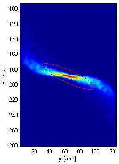
of particles is shown in figure 2.3. The curved tails of the distribution are from

the space charge forces in the electron bunch and are typical of what is seen

(36)

[image:36.595.162.471.73.357.2]

Figure 2.2: The relation between statistical measures and Twiss parameters

experimentally. Figure 2.3 demonstrates that in some cases an rms ellipse does

not describe the core of the distribution very well, particularly when the

distri-bution has outlying points. For this reason it is desirable to know the shape of

the distribution in trace space, in addition to the emittance, as the tails can be

responsible for beam loss or low gain FEL lasing for example. Therefore when

the distribution of particles in trace space becomes very disorganised,

measur-ing rms emittance can be less meanmeasur-ingful.

To add additional confusion, the terms trace and phase space are often used

interchangeably, so it is important to note the method of calculation and the axes

used on graphs. However, in most situations the numerical difference between

trace and phase space is negligible. Throughout this thesis the term phase space

(37)

[image:37.595.212.405.90.356.2]

Figure 2.3: Trace space ellipse superimposed onto a particle distribution

2.1.6 Thermal Emittance

When the emittance of a real system is measured, the thermal emittance is

al-ways included. This is the source emittance that is present at the cathode and

imposes a lower limit for the normalised emittance that can be achieved by an

injector. The normalised rms thermal emittance depends on the emitting area,

the momentum distribution, and the angular distribution of the emitted

elec-trons. The energy and divergence distributions are functions of the cathode

ma-terial and photon energy (for photocathodes). To create an accurate model of a

specific photocathode, it is important to understand the photoemission process

in that particular material. Typically, the thermal emittance is measured from

experiment, usually of the order of 0.5µm, and this value can be used in mod-elling. The thermal emittance becomes important when striving for sub-micron

total emittances in the region of FELs. The total emittance is a combination of

(38)

The laser spot size can be set to reduce any emittance growth in the low energy

region due to space charge forces or RF components. The thermal emittance can

be calculated by assuming the electrons from the cathode are emitted uniformly

and isotropically, within a radiusr in the presence of an accelerating field. The angular distribution, x0_{, then has a Maxwell-Boltzmann distribution and} _h_x02_i

can be calculated askT /mc2_{, where the cathode is at a temperature}_T_{, and}_h_x2_i₌

σ2

0 =r2/4[21]. Inserting into equation 2.14 withhxx0i= 0yields the expression

for thermal emittance, equation 2.16.

εth,n,rms=σ0

s kT m0c2

=σ0

s Ekin

m0c2

(2.16)

where σ0 is the rms of the emitting area (m) and Ekin is the average thermal

energy (eV).

2.1.7 Emittance Compensation

Although it is not possible to reduce the thermal emittance once the electrons

have left the cathode, it is feasible to minimise the emittance growth from

lin-ear space charge forces. Emittance growth from the cathode is a combination of

space charge forces in the bunch and transverse components of the accelerating

field. Carlsten [22] notes that by careful positioning of a lens, it is possible to

eliminate the emittance growth due to linear space charge in the bunch after a

drift. This assumes that, to first order, the transverse space charge forces act

as a defocusing lens. For a typical Gaussian electron bunch the strength of the

defocusing depends on the longitudinal position in the electron bunch, as the

space charge is strongest in the middle of the bunch and decreases towards the

ends. The compensation can be seen if the slice emittance of the distribution is

used. The slice emittance is calculated by dividing the electron bunch up into

slices longitudinally from tail to head. The emittance of each slice is then

(39)

solenoid at two different locations is shown in figure 2.4. The phase space is

plotted at a distance of 70cm from the cathode and 108cm where the emittance

is smallest in this case. The beam has been divided into 6 longitudinal slices

and the ellipse drawn for each of these. Figure 2.4 (a) shows that the ellipses

are all at different orientations, whilst the ellipses in the compensated case (b)

have very similar angles except those from the very head and tail of the

dis-tribution. The minimum total emittance occurs as these slice ellipses all align.

Variations in the energy distribution along the electron bunch, and non-linear

space charge forces that act on the extremes of the distribution, contribute to

incomplete compensation.

Figure 2.4: Phase space and slice emittance ellipses of a non compensated (a) and a compensated (b) beam

2.1.8 Longitudinal Emittance

In a similar fashion to the transverse emittance, the normalised longitudinal

emittance can be calculated using:

εn,z,rms = 1

πm0c

q

< z2 _{>< p}2

(40)

2.1.9 Brightness

The concept of emittance can be extended to include longitudinal bunch

infor-mation of the current density. This is called the brightness of the beam or bunch

[23], and is defined as:

Bn=

2I π2_ε

n,xεn,y

(2.18)

Bnis the normalised brightness (A/m2). Again, the factor ofπis generally

omit-ted. I is the current in the bunch and eitherIpeak (peak current) orIavg (average

current) can be used to give peak or average normalised brightness respectively.

The following section will show the importance of having a high peak current

for high gain FELs and that a high average brightness is required for oscillator

FELs. It is clear from equation 2.18 that a combination of small emittance and

large current will result in a high brightness beam.

2.1.10 Usage

For injector simulation usually the normalised rms geometric, or phase space

emittance, is calculated to give meaningful results from the modelling. It is

important to note whether the emittance is calculated at a particular time or

po-sition. Experimentally, it is normally the trace space emittance that is measured

at a particular longitudinal position. Therefore the electron bunch is projected

onto a transverse plane as it passes through that location, for example when it

hits a view screen. The emittance measured can consequently be slightly

dif-ferent from that simulated at thetimethe centre of the bunch reaches that same

location (as there is some longitudinal distribution).

Care should also be taken when using the trace space emittance as it can display

non-physical behaviour in regions with large energy spread or divergence [24].

Since in real systems it is the trace space emittance that is commonly measured,

simulation should be checked to see that the difference between phase and trace

(41)

Optimising the emittance depends on the application. Sometimes the slice or

some percentage of the beam emittance is a more useful measure of beam

qual-ity. This can, for example, be important for short wavelength amplifier FELs

where it is thought that only part of the electron bunch contributes to the lasing

process.

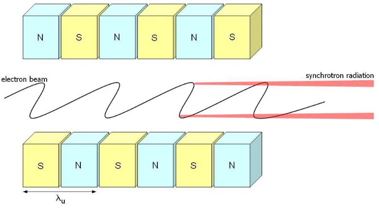
2.2 FEL Theory

In a free electron laser, relativistic electrons propagate through a spatially

pe-riodic, alternating (transverse) magnetic field, superimposed with an optical

field. The optical field can either be seeded (from a laboratory laser or another

synchrotron radiation source), or generated spontaneously from the electron

beam itself. The periodic magnetic field is provided by either a wiggler or

un-dulator. The undulator field causes electron bunches to oscillate transversely

[image:41.595.118.507.436.650.2]

and spontaneously emit synchrotron radiation, as shown in figure 2.5.

(42)

The forward radiation from an undulator is emitted in a cone of angleθ ∼ 1 γ,

and has a peak, or resonant, wavelength of [25]:

λr =

λu

2γ2(1 +

K2

2 ) (2.19)

K = eBuλu 2πmec

, γ = E

mec2

whereλu is the undulator period (m), K the undulator deflection parameter, γ

the resonant energy,Ethe electron energy (eV),Buthe undulator peak magnetic

field (T),cthe speed of light (ms−1_{), and}_e_{the elementary charge (C).}

As the electron bunch propagates through the undulator, the transverse

mo-tion of the electrons couples to the transverse electric component of the optical

field, giving rise to energy transfer. If the relationship between the electron and

electric field is correct, the optical field gains energy from the electron motion.

Whether the electrons absorb from, or relinquish energy to the optical field

de-pends on the phase. If the electron bunch is input into the undulator at the

res-onant energy, the electrons have a random phase distribution along the bunch,

so initially both processes occur simultaneously resulting in no net FEL gain.

The energy transfer gives rise to an energy density modulation of the electron

bunch, which in turn causes longitudinal bunching as the path length through

the undulator is energy dependent. The increased bunching results in more

co-herent emission, which induces more bunching, and so on, until the modulation

reaches a maximum, and the emission is fully coherent. Since most of the

elec-trons within a very short bunch have very nearly the same phase they emit with

a high degree of coherence. The average phase between the optical field and the

electrons actually remains constant as the electrons pass through the undulator

because they slip back one radiation wavelength every undulator period. This

occurs because of the longer path length encountered by the electrons and their

(43)

FELs can be configured in two ways, either as an amplifier or an oscillator. In

an amplifier, as its name suggests, the spontaneous radiation is amplified as it

passes through the undulator on a single pass. For the radiation to reach

sat-uration, the undulators need to be long enough for this to occur. Saturation

occurs when electrons that have given energy to the optical field begin to

reab-sorb it. With an oscillator, or low-gain FEL, the radiation is partially confined

between two mirrors either side of the undulator, so that it traverses the FEL

cavity many times, interacting with the electron beam. Because of the

require-ment for mirrors, the oscillator can only be used for radiation which can be

reflected efficiently, making it difficult to realise areas of the short wavelength

spectrum beyond the UV using this method [10]. In a low-gain FEL the

undu-lator is relatively short and to achieve maximum gain, the electrons should be

injected at an energy slightly higher than the resonant energy. Roughly 25% of

the radiation emitted in a single pass is permitted to escape the optical

confine-ment, whilst the remaining portion sustains the FEL process. Saturation in this

situation occurs when the power extracted from the electron beam equals that

coupled out from the optical cavity.

In the first experiments, the FELs in the amplifier (high-gain) configuration were

seeded with input lasers to begin the FEL process. It was later realised that an

electron beam instability (i.e. noise within the electron bunch) could result in

the spontaneous exponential growth of radiation to a high gain regime

with-out a seed laser. In this scenario, the portion of the spontaneous emission that

fulfils the resonant lasing criteria (i.e. equation 2.20) is amplified along the

un-dulator. This mode of operation, termed Self Amplified Spontaneous Emission

(SASE), gave the potential to extend FEL sources to the higher energy end of the

spectrum. The undulators for high-gain FELs tend to be very long so that

satu-ration can be achieved. The interaction between the radiation and the electrons

again causes a charge density modulation as some electrons gain, and others

(44)

the electron bunch length, and so results in micro-bunching on the scale of a

radiation wavelength within the electron bunch.

2.2.1 Gain Degradation

The gain of a FEL can simply be determined by the ratio of electron beam power

to optical laser power. The strength of coupling between the electron beam and

the optical field is given by the small gain coefficient (single-pass, continuous

electron beam with negligible energy spread and transverse emittance).

Follow-ing reference [26], for a planar undulator this is:

g0 =

16π γ λrLu

J IA

N_u2ξF(ξ) (2.20)

ξ = 1 4

K2

1 +K2_/₂, F(ξ) = (J0(ξ)−J1(ξ)) 2

where Lu is the undulator length, Nu the number of periods, IA is the Alfv´en

current (17kA for electrons),J the current density, andJk are Bessel functions.

It can be seen from equation 2.20 that the gain is proportional to the peak

elec-tron beam current and inversely proportional to beam energy. In real systems,

beam emittance and energy spread degrade the quality of the FEL interaction

by reducing the gain per unit undulator length. The maximum ideal gain from

a system isGmax = 0.27πg0 [26]. By correlating the effect of gain degradation

with electron beam parameters it is possible to determine the criteria for

elec-tron beam quality [27]. Typically the normalised transverse emittance must be:

εn,rms ≤

γλr

2π (2.21)

where γ = _√1

1−β2 and β =

v

c. This implies for lasing at nm wavelengths, a

(45)

energy of the electron beam the requirements on emittance become less

strin-gent. However, not only is the wavelength dependent on electron energy, but

also the small signal gain is inversely proportional to it, which would lead to a

weaker coupling of the FEL process.

2.3 Conclusions

Low emittances are required for lasing, and the shorter the FEL wavelength,

the smaller the emittance needed. The small emittance from the cathode must

therefore be preserved through the accelerator until it reaches the FEL. The

out-put power from a FEL is proportional to the current of the electron bunch, so

this must be simultaneously maximised. A high peak current implies a high

charge density which increases the FEL gain.

The emittance and brightness are limited by a number of contributing factors.

One factor is the thermal emittance of the electron source. The thermal

dis-tribution of the emitted electrons determines the lower limit to the achievable

emittance. There are also the space charge forces within an electron bunch, that

act to expand the bunch in the first stages of acceleration, before the

relativis-tic effects at higher energy make space charge negligible. This process works

in both longitudinal and transverse planes and becomes worse with increasing

bunch charge. The transverse forces are not entirely linear, and so cannot be

compensated for fully with the use of solenoids. A final consideration is that all

electrons within a bunch do not experience the same accelerating electric fields

from RF cavities. This gives rise to an energy spread along the electron bunch.

The trade-off between charge density within a bunch and the emittance must

be carefully balanced within the injector. Higher charge densities are beneficial

to the lasing process, as are low emittances. However at the low energies in

(46)

charge forces. A poor emittance in turn will degrade the lasing process in the

(47)

C

HAPTER

3 High Brightness, High Average-Current

Electron Sources

The production of electrons for acceleration can be achieved in many ways,

from traditional thermionic guns to novel combinations of photo and field

emis-sion sources. A brief overview of these electron sources is given in the following

sections.

Once electrons have been produced they must then be accelerated by an electric

field, and so all cathodes have an applied field at the surface to move the

elec-trons in the required direction. Again, methods vary for different applications.

The most common for use within an ERL or other high brightness machine are

discussed in this chapter.

3.1 Electron Sources

Cathodes can be generalised as surfaces that emit electrons under the influence

of some stimulating energy. This energy could be in the form of heat, light,

ki-netic energy from incident particles, or alternatively, the electrons may be

(48)

geometry. For example there are hot cathodes, cold cathodes, photocathodes,

field emitters, secondary emitters, and hollow cathodes to name a few. Ideally

the cathode should emit electrons freely and plentifully with zero momentum

spread, and should have an infinite lifetime.

3.1.1 Thermionic Sources

Thermionic emission is the oldest method of liberating electrons from a

mate-rial. Electrons are effectively evaporated from a heated surface. To escape the

material, electrons must have a component of velocity perpendicular to the

sur-face through their kinetic energy. The kinetic energy of an electron must be at

least equal to the work done in passing through the surface. This minimum

en-ergy is known as the work function,φ(eV), and is material specific. The work function is the minimum energy needed to remove an electron from a solid to a

point immediately outside the solid surface. The energy to overcome the work

function arises purely from the thermal energy of the system. The saturated

emission from a heated cathode is given by the Richardson/Dushman

equa-tion:

J0 =A0T2e −eφ

kT (3.1)

Where J0 is the saturated thermal emission current density (A/mm2), A0 is

Dushman’s constant (the theoretical value is 120.4 A/cm2_/K2 _{which is not}

at-tained for real materials [28]).kis Boltzmann’s constant (8.6×10−5 _eV/K),_e_the

charge of an electron (eV) andT is the cathode temperature (K). Current is de-pendent on both the temperature and the emitting area of the cathode, as is

ther-mal emittance (discussed in chapter 2). A good cathode however, will produce

a high current and a low thermal emittance, so there is a trade-off to be made.

Equation 3.1 does not take into account any electric field at the cathode surface

that is applied to accelerate the electrons away. As a result, a voltage (from an

anode adjacent to the cathode) or electric field must appear in the equations. It

(49)

emission increases. The applied field reduces the energy barrier that an electron

must overcome in order to escape the surface. In effect the work function is

re-duced byq eE

4πε0, whereE is the applied field andε0 is the permittivity of free space. The emission is therefore given by:

J =J0e

q

eE

4πε₀

(3.2)

Thermionic sources are simple devices and avoid the need for the complex

laser drive systems required for photocathodes, and as a result remain

popu-lar in some laboratories. However producing flexible, high peak current pulse

trains is difficult, as electrons are constantly emitted from the cathode surface.

Pulsed electric fields can be used to suppress emission from the surface, but

there are limitations on the repetition rate and duty cycle resulting in relatively

long pulses (∼ns). Therefore a significantly more complex injector stage is

re-quired to reduce the bunch length. Nevertheless, a thermionic gun has been

used for the JAERI FEL [29, 30] with 230kV DC acceleration. Subsequent

com-pression stages are used to shorten the bunch length. Such an electron source

has also been proposed for the Spring-8 Compact SASE Source (SCSS) with DC

acceleration to 500keV [31]. The cathode is pulsed to produce 1.6µs (FWHM) 500keV bunches, which are shortened by a number of bunching stages to 12ps

(FWHM) at 50MeV.

Secondary Emission

Secondary emission occurs when electrons with sufficient energy bombard

oth-ers in the lattice structure of the cathode and cause other electrons to be emitted

from the surface. For many cathode materials high secondary emission is

ac-companied by short lifetime. When a cold cathode is used, that is one which is

not actively heated, all the emission is a combination of field (discussed in the

(50)

operating temperatures to emit at all, and the presence of an electric field can

lower it further. The amount of secondary emission depends on the energy and

angle of incidence of the primary electron and also the material of the cathode

itself. Due to the emission process, the thermal energy of the electrons emitted

is lower than that from room temperature thermionic cathodes.

3.1.2 Field Emission Sources

As the electric field at the surface of the cathode is increased to the 103 _{- 10}4

MV/m level, it is found that electron emission increases rapidly [32].

Further-more, the increase is almost independent of temperature. With a high applied

field the potential barrier at the surface is very narrow, and even though the

kinetic energy is not sufficient, electrons can escape the surface via tunnelling.

This is the Schottky effect, and after onset, field emission increases

exponen-tially with applied field.

High fields at cathode surfaces can be achieved through the geometry of the

cathode. For example, needle cathodes which have very narrow tips (∼1µm) can have a field gradient on the surface of 103 ₋ ₁₀4 _{MV/m for an applied}

cathoanode voltage of just 50kV. These single-needle cathodes are being

de-veloped for use with table-top FELs [33], and use a laser to gate the electron

emission through the photo-electric effect. In this way very short pulses, that

roughly follow the laser temporal profile can be obtained [34, 35]. As an

alterna-tive, arrays of needle cathodes can be used as field emitting cathodes, see figure

3.1.

The emission from these cathodes is gated through a surface layer that locally

suppresses the field with a bias voltage [36]. To further enhance the field at the

tip, carbon nanotubes can be grown on the vertex [37]. As the emitting area is

(51)

Figure 3.1: Field Emission Array

gradients, the emittance from these cathodes promises to be excellent. As yet,

they are untested in an accelerator style gun.

3.1.3 Ferroelectric Sources

Ferroelectric materials exhibit a permanent electric dipole moment in their bulk

and can spontaneously produce electrons without an applied external

extrac-tion field. The electron emission results from spontaneous bulk polarisaextrac-tion

switching, which generates a high surface electric field that expels the layer

of compensating electrons. In changing the dipole moment, electrons can be

separated from the crystal lattice and emitted from the material. A change in

the direction of the dipole moment can be induced by the application of a

sub-microsecond external electric field, irradiation with a laser, acoustic waves or

heating. The use of a laser to stimulate electron emission is the most

promis-ing method of producpromis-ing short electron pulses, however the shape of emission

is not directly controlled by the laser. The electrons are not produced via the

photoelectric effect so the wavelength need not be matched to the cathode. An

example of such a cathode being used in an RF gun is given in [38]. In this

sce-nario the current produced is high, the duty cycle is low, and the pulse length

A high average current electron source for the Jefferson Laboratory free electron laser