A study of statistical growth models and growth database

A study of statistical growth models and growth database.

VEKKATESWARLU, P.

Available from Sheffield Hallam University Research Archive (SHURA) at:

http://shura.shu.ac.uk/20476/

This document is the author deposited version. You are advised to consult the publisher's version if you wish to cite from it.

Published version

VEKKATESWARLU, P. (1993). A study of statistical growth models and growth database. Masters, Sheffield Hallam University (United Kingdom)..

Copyright and re-use policy

J S & ^ I Sheffield Hallam University Hallamshire Business Park Libra 100 Napier Street

ProQuest Number: 10701123

All rights reserved

INFORMATION TO ALL USERS

The quality of this reproduction is dependent upon the quality of the copy submitted.

In the unlikely event that the author did not send a com plete manuscript and there are missing pages, these will be noted. Also, if material had to be removed,

a note will indicate the deletion.

uest

ProQuest 10701123

Published by ProQuest LLC(2017). Copyright of the Dissertation is held by the Author.

All rights reserved.

This work is protected against unauthorized copying under Title 17, United States C ode Microform Edition © ProQuest LLC.

ProQuest LLC.

789 East Eisenhower Parkway P.O. Box 1346

A STUDY OF STATISTICAL GROWTH MODELS

AND GROWTH DATABASE

P VENKA TESWARL U

A thesis submitted to Sheffield Hallam University

in fulfillment of the requirements for the degree of

Master of Philosophy

Sponsoring Establishment

International Crops Research Institute for the Semi-Arid Tropics, Patancheru

Andhra Pradesh 502 324, India

Chapter 1 Chapter 2

Chapter 3

Chapter 4

Chapter 5

Chapter 6 Chapter 7

CONTENTS

Page

Introduction 1

Statistical Modeling 3

2.1 Introduction 3

2.2 Purpose and Types of models 4

2.3 Criteria for models 6

2.4 Methodologies for modeling 8

Plant Growth Models 13

3.1 Introduction 13

3.2 Polynomial growth models 13

3.3 Growth Data 15

3.4 Fitting Growth Models 27

Application of Growth Models 29

4.1 Introduction 29

4.2 Analysis of Variance 34

4.3 Fitting Growth Models 43

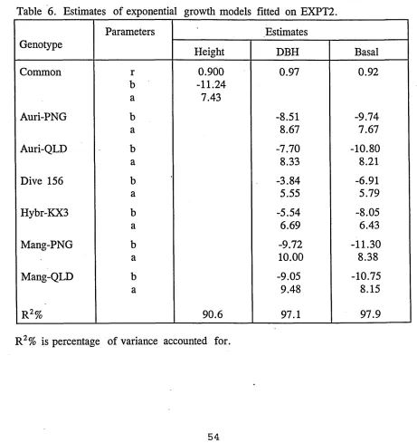
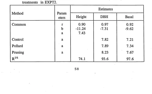
4.3.1 Exponential curves over genotype and cutting 44 combinations in EXPT1.

4.3.2 Exponential growth models for genotypes and 53 cutting in EXPT2.

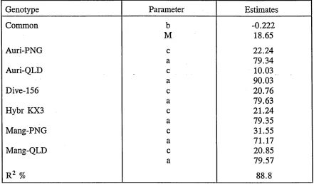
4.3.3 Logistic growth models for genotypes 61 A Growth Database - GROWDAT 64.

5.1 Purpose of Growth Database 64

5.2 Structure of Growth Database 64

5.3 Future Plan of Work 65

Conclusion 66

References 68

A STUDY OF STATISTICAL GROWTH MODELS AND GROWTH DATABASE

P Venkateswarlu

Plant Physiologists and crop modelers in general are keen to use non-linear models for their work. However, usual practice remains restricted to the use of linear form of growth curves due to lack of proper methodology for the application of non-linear models.

This study is undertaken to review the statistical literature available on non-linear models, comparison of these models with data sets available.

ACKNOWLEDGEMENTS

I would like to express my sincere thanks to Dr G K Kanji, my first supervisor for his encouragement to undertake the work and for all his invaluable help during this study.

My sincere thanks and profound gratitude are due to Dr. Murari Singh, my second supervisor for his full support and guidance during my study.

I also thank several physiologists at the International Crops Research Institute for the Semi-Arid Tropics, Patancheru, India, who have extended their valuable suggestions for the development of growth database.

1. Introduction

A clear idea of development behaviour of plants is essential for human endeavour

to improve them. Often plant scientists are interested in selecting an ideotype or a

genotype with a desired growth behaviour, to cope up with various stress factors

anticipated over a specific time interval and yet maintaining acceptable yield levels.

In order to study the plant growth, experiments are conducted on desired genotypes

of the plant and with a set of treatments applied on them, a sequence of response

(such as height, diameter, drymatter etc.) are recorded over the growth period.

Using the record of the response over time points, a functional form of the growth

is evaluated. The parameters of the function are interpreted from biological or

physiological points of view. These parameters are the characteristics of the plant

genotype and the treatment (if any) applied on these genotypes. The selection of the

genotype and the treatments is then done on the basis of the estimates of the

parameters of the growth functions or the curves.

A number of models or functional forms for the plant growth will be reviewed in

chapter 3 and the philosophy behind statistical modelling in chapter 2. It is quite

essential to realize that in practice, we generate responses based on experiments

conducted in field, green houses, plastic house, laboratories or incubators. These

responses therefore have a component of experimental error. In order to make a

.to follow principles of experimental designs advocated by Sir R. A.Fisher. Once the

responses have been obtained they are better explained by models which incorporate

stochastic components. Such models are called ’Statistical Models'. When the

stochastic component is ignored, we have the deterministic models. The statistical

models are relatively more realistic and if a suitable procedure for estimation of

model parameters is followed, one can assess the reliability of the estimates.

A set of eight experiments from humid sub-humid trials of Forest/Fuelwood

Research and Development Project, Bangkok, were conducted on Acacia auriculiformis, A. mangium and Leucaena trees. Summary of the growth behaviour of the genotypes and cutting management treatments on height, diameter at breast

height and survival percentage are presented in Chapter 4.

The study of plant growth is an essential component of research in physiology. The \

data sets for such research are in the form of time series and differ from the data

sets of those plant disciplines which require one time observations on experimental

units (generally at final stage, e.g. yield of a crop at maturity). Due to this

specialized nature of data set, an appropriate software for the data storage, editing,

retrieval and analysis becomes necessary. In Chapter 5, Growth database developed

in dBase III is presented. The instructions for using GROWDAT are presented in

2 Statistical Modelling

2.1 Introduction

It is an approach and more than just a collection of techniques and models.

As noted by Meadows (1980): " Statistical modelling should be considered a

paradigm in understanding in a similar way to that in which systems dynamics

or econometrics can be considered"

The following elements may be considered as essential to the statistical modelling

approach

1. The inherent randomness of systems and in consequence all data will contain variability.

2. Importance is attached to data, and data should be handled consistently.

3. A wide range of modelling skills will be required in addition to statistical skills.

4. The main objective is gaining insight into the situation being studied.

5. Statistical techniques will be prominent in the above.

Statistical modelling is an approach that can be applied to any area. Although it is

most readily applied to ’hard’ scientific studies and it can also be applied to ’softer’

2.2 Purpose and Types of Models

It is essential to understand the precise meaning of the following questions

Do I need a model?

What type of model do I need

What approach to modelling shall I take? What are the steps in modelling?

in order to model any behaviour.

Models come in many different forms. These can be considered as a subset of

symbolic models in Ackoff and Sasceni (1968) categories of Conceptual models,

Iconic Models, Analogue models, and Symbolic models

A list of reasons for using models could be that they communicate fact and ideas;

generate new ideas; predict behaviour; provide insight into the behaviour; clarify

thinking etc.

Jeffers (1982) gives various reasons for using ecological models including an orderly

and logical representation of the underlying relationships; a means of communication

between different research works; and a synthesis of available information. Thus

there are three main themes in the purposes of models

The emphasis placed on the three aspects will depend on the particular situation.

A contrast between (i) and (ii) and (iii) is often set up.

Gilchrist (1984) describes a contrast between conceptual and empirical aspects. The

conceptual approach uses "logical reasoning, ’known theory’, to obtain a model".

Whereas the empirical uses only the empirical evidence, the data. In practice a

mixture of the two approaches is used, what Gilchrist calls the eclectric approach.

In relation to the two aspects ie.,descriptive and explanatory models, is the idea of

’biologically meaningful parameters’. That is the parameters involved in a model

should have some biological interpretation. The problem with these parameters is

that the statistical estimates of such parameters often do not have ’nice’ statistical

properties, they are often complex non-linear functions of the natural mathematical

parameterization of the model (Causton and Venus (1981)). Hunt (1982) argues

caution on rejecting a model simply because its parameters cannot be given any

general biological significance. Information is often not supplied by the parameters

but through their derivatives. As Hunt states ’parameters are messengers of reality,

not reality itself. Gilchrist also considers the problem of reality, ’a model is only a

limited, and possibly distorted, picture of reality’. " A model can be seen as truth

insofar as it makes ’unhidden’ aspects of the situation being modelled that were

previously hidden". He goes on to say that the important aspect is the adequacy of

.When one looks at a flexible function such as the Richards function the empirical-

mechanistic divide seem even fuzzier. It is a mechanistic model because it comes

from a certain differential equation model with possible mechanistic interpretations?

Or is it just a useful empirical model? Obviously the fit of the model alone does not

necessarily imply the underlying mechanism. There has to be an interpretation of

the mechanism, but how satisfactory does it need to be? There are general ideas

about growth behind the models considered but are these ideas good enough for any

situation?

There is a second problem with flexible models, that of falsification. The concept

of a hypothesis or model being falsifiable is central to the standard scientific

approach. If a model is very flexible then it becomes difficult to falsify it, so it is

always right. For some model such as splines this is not a problem because no

interpretation is placed on them, they are purely smoothing functions. For some of

the generalized logistic models there is an implicit mechanism behind them. How

useful are these ’always right’ models. This brings us to the next subject to examine,

criteria for models.

2.3 Criteria for Models

What makes a good model? Randers (1980) listed the following desirable

a. Insight generating capacity b. Descriptive realism

c. Mode reproduction ability d. Transparency

e. Relevance

f. Ease of enrichment

g- Fertility (or new ideas, experiments etc) h. Formal correspondence with data

i. Point predictive ability

These criteria were primarily set up from a systems dynamics viewpoint. The above

can be used to set up some general criteria which may be more in sympathy with

statistical modelling.

A. Data Correspondence

Does the model make use of all the available data? Is its use of data

consistent, making use of pre selected criteria to judge closeness of fit.

Have regions of inadequate data fit been shown to have no substantial

effect on the overall model?

B. Justifiability

Is the complexity of the model required? Can the model be falsified

given the quantity of information available? If not, is the model

C. Applicability

Can model predict behaviour if required? Is it relevant to the end

user?

D. Insight

Does the model increase understanding of the modelled system? Does

it indicate areas of inadequate understanding?

2.4 Methodologies for Modelling

The idea of statistical modelling as a subject has grown considerably in the last few

years. Following are the steps to be considered for statistical modelling as suggested

by Gilchrist (1984):

1. Identification

Selecting the most suitable model. The identification may be based on ideas

about the situation (conceptual), the data (empirical) or a combination of

both.

2. Estimation and Fitting

The parameters of the model are estimated using suitable criteria and the

3. Validation

The validity of the model is considered, this can take place at various stages

in model development.

4. Application

The use of the model, this will effect all stages of the modelling process.

5. Iteration

The above stages are not linear but the modeler will pass back and forth

between them.

This approach works well in areas such as linear regression modelling and time series

modelling in which you are dealing with a well defined family of models and

selecting the best from that family. If a broader view is taken and the subjective

nature of the modelling process is to be fully considered then a modified

methodology is required.

Several problem solving methodologies have been developed for soft systems ie

systems involving qualitative variables and subjective judgement. One such

methodology is due to Checkland (1972). The essential stages are

(a) Analysis

(d) Comparison of definitions of possible changes (e) Selections

(f) Design and implementation (g) Appraisal

These stages can be seen as (i) obtaining information about current systems; (ii)

reducing the system to its basic purposes; (iii) constructing models; (iv) comparing

results of models with the situation to suggest changes which can then be selected

and applied.

Using the ideas of this methodology a new methodology for statistical modelling can

be developed.

(1) Conceptual Analysis

The object of this phase is to produce a conceptual or ’ideas’ model of the

situation to be examined. It will contain all possible relationships and their

forms and the data available. The use of diagrams such as system maps and

influence diagram are an important tool at this stage.

(2) Model Type Generation

Using the insight gained from (1) a number of possible types of model to be

used are considered (eg stochastic differential equation models, linear

(3) Model Building

At this stage the models for each type are constructed. Within this stage

Gilchrist’s methodology (1-3) can be used for each model type. A single

model need not emerge from each type as there may be several competing

models with little objective distinction between them.

(4) Comparison of Models

The models from (3) will be compared with respect to both direct application

and generated insight. This comparison will primarily be a subjective

comparison.

(5) Generation of Further Model Types

As a result of (4) improved models may be suggested.

(6) Application and Appraisal

The results of the above model will be used and critically evaluated.

The above methodology can be placed within the modelling-data collection circle and

one of the applications may be data generation. It is hoped that such a methodology

will lead to a more flexible approach to statistical modelling.

criteria guiding the models and conceptual steps in identifying the models. In the

following chapter, emphasis is given on the models specific to the study of plant

3. Plant Growth Models

3.1 Introduction

Linear models have dominated the statistical methods for investigating relationships

not because such models are always the most appropriate but because the theory of

fitting such models to data is very simple. The calculations involved in obtaining

estimates of the parameters in linear models requires only the solution of a set of

simple simultaneous equations.

In contrast more realistic forms of models which involve parameters in a non-linear

fashion cannot be so simply fitted without the use of a computer. Some forms of

nonlinear models were investigated before the development of modem computers,

and the complicated methods of fitting them were devised later. However these

models inevitably had little appeal to research workers and were not widely used in

the past because of their complexity. With the availability of high speed computers

the fitting of non-linear models should be no longer difficult than that of linear

models. It is therefore important that the research biologist should be aware that

there would be no difficulties in fitting these models.

3.2 Polynomial Growth Models

why linear models are inadequate to biological situations. If we are considering a

relationship between a stimulus variable, X, and a resulting yield variable, Y,

then the three simplest forms of linear models are the straight line Y = a

+ bx, the quadratic form Y = a + bx + cx2, and the cubic form Y = a + bx

+ cx2 + dx3. These are special cases of polynomial curves.

The straight line is obviously a very restricted relationship. Very few biological

relationships are even approximately straight for a reasonable range of x values. The

most common form of straight line relationship being, perhaps, the allometric

relationship between the logarithm of weight of a plant or animal part and the

logarithm of the whole plant or whole animal weight.

The quadratic model allows for curvature but is restricted in two critical ways. First,

it is symmetric, the size of Y with increasing x to a maximum being of exactly the

same form as the subsequent decline of Y with further increase in x. The symmetry

can be avoided by considering not x but a power of x. Y = a+b(x°)+c(x°)2

which is often a useful form of model, but is now a nonlinear parameter. The second

disadvantage of a quadratic model is that the value of Y must become negative when

xis either large or small and this will usually be biologically unreasonable. The cubic

polynomial, and polynomials of yet higher degree overcome the disadvantage of

symmetry but not those of producing unrealistically negative or very large values of

.maximum and minimum values.

None of the curves in the polynomial family of models allows for a relationship

which tends to an asymptotic level of Y as X becomes large, or relationships where

Y is necessarily positive. In contrast, most of the nonlinear models in common use

do allow such biologically realistic forms of behaviour. In addition, many of the

commonly used nonlinear models can be derived from simple biological concepts

which to the extent that they are appropriate, justify the use of the non-linear models.

3.3 Growth Data

Data on the growth of part, whole or groups of organism are collected in many areas

of biological sciences. In agriculture or forestry the growth of crops/trees and

animals is studied, in medicine it is the growth of individuals or the growth of tumors,

and in botany the whole plant can be looked at or one can look at a particular part,

for example a leaf or tiller.

Many biological investigations are also concerned with the growth or organisms with

time. Extensive studies have been made of the growth of whole plants, or of the

growth of the individual leaves, or of the growth of the animals. Qualitatively the

growth of a biological organism can be thought of in four stages. Early growth,

quantitatively by saying that the rate of growth is proportional to the size of the

organism. This form of growth is often called ’exponential growth’. If the rate of

growth is exactly proportional to size then the size of the organism is described by

the exponential function. The second stage is relatively less rapid, as more the

energy of the organism is devoted to maintaining the current size. During this stage

the growth of the organisms may well be approximated by the linear relationship.

The third stage, the organism’s growth diminishes further as a balance between the

energy of the organism and the maintenance requirements is approached. The fourth

and final stage of the growth is the antithesis of growth.

These above names were first used by Causton (1967); Rodford (1967) used the term

’dynamic’ for what we call the ’functional’ approach but terminology is relatively

unimportant provided it is realized that one approach necessarily involves the use of

fitted curves and the other does not. The classical approach in which the course of

events is followed through a series of relatively infrequent, large harvests with much

replication of measurements, the functional approach in which harvests, supplying

data for curve fitting are smaller (less replication of measurements) but more

frequent.

The data collection can be classified into two groups. The first is when a single

entity is studied through time and measurements are taken at various times. The

•in order to study the growth of the population as a whole. This is common in the

study of crop growth when for example, in studying grass growth over a season a

sample of grass given by a randomly placed quadrant would be harvested and

weighted every week. One of the particular difficulties with the type of data,

especially with the first type of collection, is that the observation will, in general, not

be independent but correlated (Morgan, 1986 ). Glasbey (1979) considers five

contributions to the errors of a model of the growth Ayrshire steel calves.

a. Variations in grid fill between weightings.

b. Seasonal variations and changes in diet

c. Illness

d. Errors in measuring procedure

e. Choice of wrong biometric form of the curve.

Of these b, c and e result in correlated errors.

In the case of sampling from a experimental population changes in the environment

which would be common to the samples would also lead to the correlated error

structure. Thus while standard regression modeling procedure involve the

assumption of independent errors this will rarely be valid in the case of growth data.

.standard shape being that of a sigmoid curve, thus the most natural model form is

a not linear model.

There are three basic approaches to this problem. One is to consider functions of

the observations, usually some form of differences, and assure that these are,

approximately independent. Some form of analysis is then carried out on these

functions of data (Radford, 1967); Hunt, 1978,1982).

Alternatively, a second approach which will be called the statistical approach, relies

on approximating the growth curve by a low order polynomial. The advantage of

using a polynomial is that it is statistically simpler to deal with and a procedure

involving a general error structure can be arrived at which only involves linear

computations. However, it is rarely possible to assign a biological meaning to the

parameters of the fitted model thus making interpretation difficult.

The third approach is to fit non-linear models whose parameters have a reasonable

biological interpretation. Being non-linear these models involve greater problems in

estimating the parameters than do the linear models. Numerical techniques have to

be employed in order to minimize the resulting non-linear sums of squares function

required by least squares procedure. Also little work has been done on fitting non­

3.4 Fitting Growth Models

The following asymptotic functions were also examined with the data sets in addition

to fitting exponential equations. In an asymptotic function, whatever its other

properties, the form of its progression is governed by one characteristic feature: the

value of the dependent variate more and more gradually ascends (or descends) to a

plateau which it never quite meets. This plateau in the value of Y is known as the

asymptote, or asymptotic value, and is the value predicted for Y when X is at infinity.

Though this property of asymptotic functions is universal, it is not necessarily obvious

in the form of every fitted progression. Unlike the polynomial functions, the

asymptotic functions are statistically non-linear.

1. Monomolecular function

2. Logistic

3. Gompertz

4. Richards Function

3.4.1. Monomolecular function. The monomolecular function is described

mathematically as

.where a is the asymptote, b a measure of the starting size of the system ari c i s

rate constant. The above equation is the basic function fitted to untransfonriec^

primary data. In asymptotic functions as in case of polynomials, asymptotic finctio^

can also be subjected to logarithm transformation for the mathematical puipose

linearizing or simplifying the function to secure an easier method of fitting

Transforming both sides to logarithm produces

logeW = logea + loge(l-b e'cT) . . 1.2

Here the parameter retain their original relationships vis-a-vis with

untransformed data and the growth function iteself becomes simpler with

changed properties (Causton, 1977). Transforming the left hand side only

logew = a(l-be*cT) . . 1.3

an equation which following the terminology adopted for polynomials by Causton

(1970) may be termed the monomolecular exponential. This may be done in c^ses

where the logarithms of primary data are homoscedastic and lie in a progression, ^

general shape of which corresponds broadly to that of the function. The structJre

and properties of the function are not altered by this transformation. It is me;ejy

applied to the logarithm of data instead of to their arithmetic values,

•reason to perform subsequent comparisons on an untransformed basis. Values of

logew may require the addition of constant to remove negatively and this must also

be allowed for in a. There is an important difference between this procedure as that

in which the whole function is transformed to logarithms as in equation 1.2. In this

former case, if the experimenter is prepared to estimate and iterate around the

asymptotic values, a, the basic monomolecular function written in the form of

equation 1.2, a, may be linearized and fitted to data in the form

loge[l-(W/a)] = lo g eb-cT .. i , 4

and the same may be done for the monomolecular exponential equation 1.3

loge[l-(loge W/a)] = logeb-cT •• 1*5

Linearisation by logarithmic transformation is in equation 1.4 and 1.5, a

mathematical device which brings the non-linear function within the bounds of simple

regression methodology. But it also alters the statistical properties of the primary

data.

The monomolecular function is one of the simplest of asymptotic functions. It has

no point of inflection and its scope has a progression which is convex to the time

axis, being proportional T the amount of growth yet to be made, a‘w. In this respect

.polynomials though it differs from that function in that being genuinely asymptotic,

it is unable to proceed into negative slope.

3.4.2. Logistic function. This function is, like the monomolecular, a three parameter

function, is also known as the autocatalytic function and takes the form

W(or logeW) = a/(l+be ‘cT) .. i.e

where the bracketed term on the lefthand side refers to the dependent variate of the

logistic exponential. The value of W (or logeW) at T= 0 is a/(l+b) and the function

has a symmetrically placid point of inflection at T = (logeb)/c and W for logeW =

a/2. After linearisation the functions may be fitted in the forms

l°ge[(a/W)-l] = logeb-cT . . 1. 7

or

loge[(a/ logeW)-l] = lo g eb-cT . . 1 . 8

For the logistic the slope are

dW

and

1 dW

. ---= bce'cT/(l +be -cT)

W dT

and for the logistic exponential

dW abce[a/(l +be cT)-cT]

dT (1 + be-01)2

and

1 dW abce ‘cT

W dT (l+be*cT)2

The logistic equation has been used very extensively in the field of animal ecology

for the modeling of change in numbers of individuals within a population (Solomon,

1976).

3.4.3. Gompertz Function. This function devised by Benjamin Gompertz in 1825,

also has three parameters but these are arranged as a double exponent.

W(or logeW) = ae‘be 'ct . . 1.13

The value of W(or logeW) at T = 0 is ae'b. Like the logistic the Gompertz’s point

of inflection occurs at T = (logeb)/C but in the W (or logeW) dimension the curve

.. 1.10

.. 1.11

.is asymmetrical with an inflection at a/e. The linear arrangements for the purposes

of fitting are, for the Gompertz.

loge[loge(a/W)] = logeb-cT .. 1.14

and for the Gompertz exponential

. 1.15 V V ■■ • 1 IV I l«l . ■

j e * - t o e

I0ge[l0ge(a/l0g eW)] = l0geb-cT

In both cases, the double logarithmic transformation is necessary to eliminate the

double exponentiation present inequation in 1.13. The derivatives of the Gompertz

are

dW

= abce'cT'be .. i .i6

dT

and

dW

= b c e'cT •• 1-17

W dT

and for the Gompertz exponential

dW

and

1 dW

= abce . . 1.19

w

Lengthy comparative discussions of the properties of the Gompertz curve, especially

in relation to those of logistic, have been given by Winson (1932) and Richards

(1969). The former warned that there seemed to be "no particular reason to expect

that the Gompertz curve will show any wider range of fitting power than any other

three constant S-shaped curve. The degree of skewness in the Gompertz curve is just

as fixed as in the logistic and it is clear that to introduce a variable degree of

skewness into a growth curve will require at least four constants. Of the Gompertz

and logistic functions the latter wrote "since many (asymptotic) growth data are

characterized by maximal rates somewhere within the range of a/3 to a/2, these can

usually be fairly well accommodated by one or other of the two. Though this opinion

did not prevent Richards from devising himself (in 1959) what has since come to be

the most important of four parameter functions.

The majority of applications of the Gompertz function in plant growth analysis have

been connected with the modeling of the growth of individual organs, particularly

that of leaves.

•F.J. Richards in 1959, has four parameters:

W(or logeW) = a(l .. 1.20

and the second exponent, -1/d, involves the additional parameter, d. The term

is a more modem rearrangement of be‘cT, which was formerly used in this function

in the same way as in the monomolecular, logistic and Gompertz.

Derivatives of the Richards function are

dW aceb'cT

__________ = . (1+ e b-cTyi(l/d +1) . . 1 . 2 1

dT

and

dW ceb'cT

= .. 1.22

W dT d (l+ ebcT)

and for the Richards exponential

dW aceb'cT

= ^ ( l + e b-cTy(l/d+l)

dT d “ 1,23

etaC l+ e^7)-1^]

1 dW aceb-cT

. (1 +_ e ),b-cT\-(l/d+l)

. . 1.24

W dT d

The previous three functions such as Monomolecular, logistic and Gompertz, have

had linear forms which may be fitted if a value of a is first sought by trial and error.

In the case of the Richards function, the originator’s (1959) method of fitting was to

select both a and b by this method. Subsequently, a long sequence of improvements

on this approach has evolved (Nelder, 1961; Causton, 1969; Davies and Ku, 1977;

Hadley, 1978) culminating into most modem medthod of fitting which enjoys

automatically computed starting values, a separate treatment of a and d, stability of

the method over wide variety of curve types. The Richards function represent a

much wider class of growth phenomenon than over by some of the previous models

which are its special cases.

Above curves can be easily fitted using a general statistical software, such as

GENSTAT (A General Statistical Program) or SAS (Statistical Analytical Systems).

For example, GENSTAT’s FITCURVE commands has options for fitting ten

standard non-linear curves. Some of these are the models discussed in this chapter.

This chapter presented various forms (linear, polynomial and non-linear including a

major class of function known as ’Richards’ function) for modeling plant growth. In

reality, for a given plant genotype, many forms of the growth models discussed may

•presented the functions fitting well to the growth behaviour of the trees selected

4. Application of Growth Models

4.1 Introduction

Data from seven Humid and Sub-humid Zone Network Trials conducted by the

Forestry/Fuelwood Research Development Project, Bangkok, have been used for the

application of growth models. Experiments are coded as EXPT1 to EXPT7 for

convenience.

Experimental Design

The experimental design is a randomized complete block in 3 replications, using a

factorial arrangement of six genotypes or provenances x 3 management treatments.

The two factors are labelled as Genotype and Cutting management treatments.

Management treatment on each plot is applied to all live trees including trees in

buffer rows. The total number of treatment combinations are 18. The genotypes

considered in the experiment are nitrogen fixing forest trees. The characteristics of

these forest trees are presented in Annexure 1 for the interest of the readers. They

at breast height and survival percentage are recorded at an intervals of 6 months

starting from 6 months upto 36 months. The procedure of recording various tree

measurements are presented below.

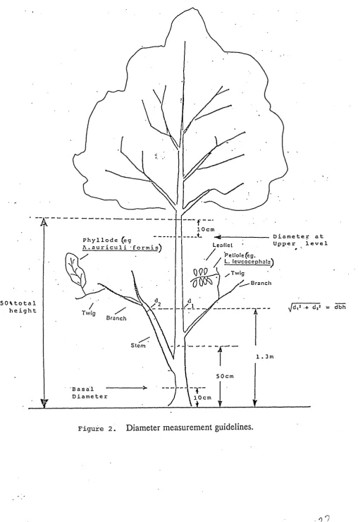
Height

Measure the total height (Figure 1). If there are multiple stems, measure the tree

from ground level to the top of its highest apical bud. If the site slopes significantly,

measure the principal stem from the uphill of the tree. If the trees are bent over,

straighten them if possible, so that the actual length of the stem is measured. Use

a height stick or some type of marked, rigid pole to take height measurement.

Basal Diameter

Basal diameter is defined here as the diameter at 10cm above ground level (Figure

2). Take measurements on the principal stem (and other stems originating below

10cm). Mark with paint the point of measurement to ensure that the same point is

measured subsequently. The measurement should be made with a metric diameter

tape or vernier caliper. For multiple stemmed trees, the average diameter is

calculated using the following formula:

da = SQRT(dl 2 + d22 + ...dn2)

branching bole is considered a stem if its diameter is equal to or greater than 50%

of the diameter of the principal bole at the same height.

Measurement should be made on the same trees used for height measurements at

the ages of 6, 12, 18, 24, 30 and 36 months.

Diameter breast height (dbh)

Take dbh measurement at 1.3 meters above ground level (figure 2). For forking

trees or trees with multiple leaders, take the dbh measurement on all stems if forking

or multiple leaders originate less than 50cm above the ground. Mark with paint all

the points of measurements. If there is an abnormality in the tree at 1.3 meters,

measure the tree diameter at the point nearest this height which is representative of

the stem’s diameter.

Survival

Survival is the number of live trees at the time of observation.

The common objective of the experiment was to assess the differences in the growth

behaviour of various genotypes and pruning treatments for above four characters.

In this chapter, we first study the variability due to genotype, cutting method and

their interaction with time, explained as polynomial contrast. In many cases simple

(a) Height measurement on a sloping site. •

S te m Height

' ' A

5 0 % to ta 1 height

T

10 cm

■

-Leaflet

/ PetIole(eg.

^ L. leucoccphala^

/Twig

/) (jSjTM I Branch

Diameter at Upper level Phyllode (eg

A .auricu1i •formis^

dbh

Twig

Branch

Stem

1.3m

5 0 cm Basal

Diameter [“T “ 10cm

attempt to fit growth curves was made and compared the related parameters of the

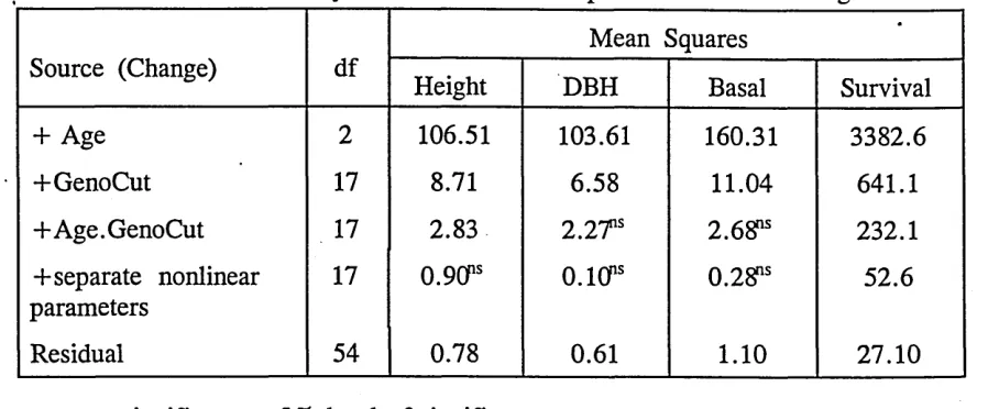
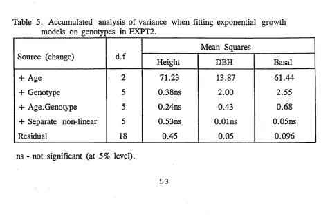
growth models. For illustration, results from EXPT1 and EXPT2 are presented in

the tables.

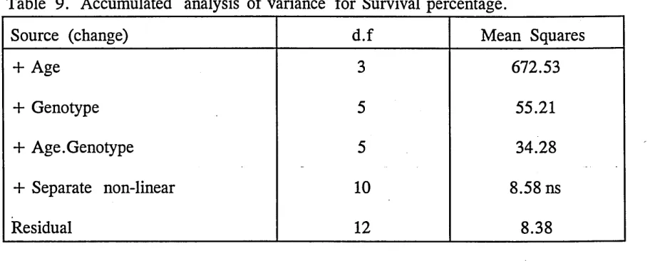
4.2 Analysis of Variance

The various induced sources were separated from the inherent sources of variation

such as replication and experimental units (experimental error or residual) using the

analysis of variance (skeleton anova shown in Table 1).

The ANOVA is of split block structure where genotype-cutting (main effects of

genotypes, main effects of cuttings, interaction effects of genotypes and cutting)

combinations are compared with an error different from that for interaction of

genotype-cutting with time. The main effects of time (age) can not be tested for

statistical significance since time can not be randomized in these experiments, but the

interactions of genotype and cutting with time have valid test due to the (restricted)

randomization of genotypes and cuttings. Summary of Analysis of variance for all

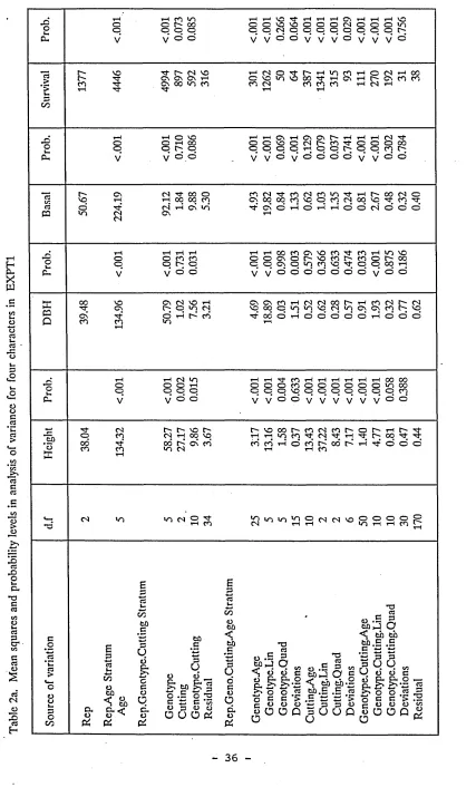
the seven experiments are presented in table (Table 2a to 2g).

Significant interactions were noticed for genotype x cutting x age for all characters

inEXPTl. Genotypic behaviour overtime was also different. Cutting methods have

Table 1. Skeleton of Analysis of Variance

Source of Variation df SS MSS

Rep r-1

Rep.Age Stratum

Age t-1

Linear 1

Quadratic 1

Cubic 1

Deviation t-4

Residual (a) (r-D(t-l)

Rep.Genotype.Cutting Stratum

Genotype _g-1

Cutting c-1

Genotype. Cutting (g-D(c-l)

Residual (b) (r-l)(gc-l)

Rep.Geno.Cutting.Age Stratum

Genotype.Age (g-l)(t-l)

Genotype. Lin _g-1

Genotype. Quad _{. g-1}

Genotype. Cubic _g-i

Deviations (g-l)(g-4)

Cutting. Age (c-l)(t-l)

Cutting.Lin c-1

Cutting.Quad c-1

Cutting. Cubic c-1

Deviations (c-l)(t-4)

Genotype. Cutting. Age (g-l)(c-l)(t-l)

Genotype. Cutting. Lin (g-D(c-l)

Genotype. Cutting. Quad (g-D(c-l)

Genotype. Cutting. Cubic (g-l)(c-l)

Deviations (g-l)(c-l)(t-4)

Residual (r-l)(gc-l)(t-l)

bl e 2a . M ea n sq ua re s an d pr ob ab ili ty lev els in an al ys is of va ria nc e for fou r ch ar ac te rs in E X PT 1

.o_o o_o h co m

C > 00

o o o c op p

V V

VO Tf

VO VO o o o c3 p p o o v v v

ON T—l _ _ cm o o o o o _o

V V V

T-I VO O to o t> _o

t"-CO rf r- CM VOCV ON CV r-t CN 00 WO CO _Tf H N O rth H i^ rO C V O V O V O O O T f r H C v

CO CM CO CO CO O M H oo h- C\ CO CO CM t—I 00

o oo 1—I O VO OHM 0 0 - 0

V o o'

H t-H CN t—I CN CN O- T—l T—l T—l CM Tt- OOvoOCNt^COrt-OOOOO C 0_ p p rH p p 0-_ 0_ O CO 0^ _{O v/O O O O v/ v/OO}

V V

C3 pa

r - C N CM 0 0 o c o CM T }- C O v q T—1 T—1 o q 0 0 C O c n 0 0 0 0 C O o T j" CM T—1 C N > d t}-’ C N O T—l v o CM

CM C N tH

T-| O T-I T-I O Oin rf CO CM 00 VC vr CO NTh o- oo cm’ o ocm' oo

o

tH o

c T—lO

O t-H

CO

f -T—l_CO o

T—l o

o T—1oo 0 0Cv

Cv

CO

o

o CNo_vovovo_COCOCO

VO

Tfr

r-TfCOCoOT—loo vor-0 0

vo 0 0

t-H

Pt _V V o o _{V V} o o o o o o o _V o o

D

B

H 0 0_TT VO

CN CvC- CoMVOvoT—1CM CNvoCvOO COo vo CT - I vo CMVOMs t"voT—lCN COCN CCMOr-~f- CVOM CN_CO ri-_co

T—l

o

votH r- CO 0 0

T—l o tH o o o o o T—l o o o

. T -I T—l CMVO T—l t-H Tf COT—l T—l T—l T—l T—l T—l C O 00

——_C o _O o t-H O O o COo o o o o o vo 00

l_ p O o o O p o vo p p p p p p o CO

PU _{V V o o ’ V V o ’ o ’ V V V V V V o o’}

Tf CM t~- r- vo r- r- VO 00 r-~ CO CM CO p r- rH C>

*tb O CO CMT—100 vq tH t-H vq co Tt CM Tf T—l cq 00 tJ-

•d-oc5 Tt 00 iS CN cd COcd tH o cd S 00 T—l t}- o o* o ’

o

*—« CO COT—l vo CM T -I T—1 CO

CM VO VO CMO Tf _{tH CO} CM CM VO O O O_{VO H T—l COo}

o-oto o

CO Pia.<D

^5 to_CW <L> ^

Pi CO to c V cc o c cL o pi u

& to _c to c P

u_ai p- « O' P o .2 o ’a c t; c •« _{O o o o} a u o pi

6 p w_rt I-w o to «;_to c p u o c o

a

o o c

03

T - 3

o .S 3 a j o « & &.2 <; tb tb .2

o o 60.5 .5 p O 3 3 .5 5Z *2 C Ot)t)T_.ppt> o O O Q p U U Q

O CJ

•O r - 3

o -S 3 to_j O < to to

to.3 .5

.3_{£J p p}o o

p U C> U O d a

i § § i i § § ° ’5 2_{r - fl) O O W}

Ta bl e 2b . M ea n sq ua re s an d pr ob ab ili ty lev els in an al ys is of va ria nc e for fou r ch ar ac te rs in E X PT 2.

.o_o o

o

r-! W O rH © © © © p p V V

y—* H IT1 O n t-H H t"' t'-' I’"* r o o r o m o o o n - T j - o o p p p p p p p c o c o p p p

O O V V O O V V V ©

V V

«

>

P co

Cn

Cn Cco_On

CO

WO vo wo CN O t o

■vt CO CN oo©wooocor-»oocNTt-cNwooot-' CtOVOtTfM(OMhNOtOH(S n ( O H T f r l CN

O O_O H Tf tO C C O 00_{o o} V o o

H H C O t O H r l c O H N V O t O O O © rt C" © © O Nf to 00 C Tf P P W O p p p p v o 0 0 rH p c n

o o v V O o o o o o

V V

C3 PQ

CN

00 r-~CNcd_{c n} CN

0 0 CN f" H O O to O CN V O rH rH CN

cNCNt^rrr'coc^oor'Ovnco t o CO H CO O t o N H H CO H H

r - 5 v d 0 0 r H c d r - 5 0 0 0 0 0

. _{rH rH VO VO rH rH rH rH rH rH rH Cnwo vo Tj-Cn}

© o CO CN C O o o o © © rH CO CN ■3-Ht

ou* p p o WO O O p p © O © © C" 00 00 CO

p- V V o © _{V V V V V V V} © cd©■ © cd

tc CN rH rH o CO 3; c VO rH CO CN vo00 rH CN vo vo rH ©

Hh _{*0 CO P CO CO TT rH CN CN vo© p © CO O © © rH rH}

PQ rH cd rH vdrH rH rH CN © o rH rH CN o O* © cd©* cd

Q rH VO CN

o rH©_© TJ-CN_© rH©_© t"₈ rH©_© rH©_© rH©_{O CN}5 rHo_© rHO_© rH©_{© ©}©rH CNVO_wo r~~rH_© worHrH C n CN

Cn

Ph _V © _V o _{V V V} O _{V V V V} © © © ©

H

ei

gh

t Cn

VO COrH OOCO rfCN COrH wovoCrHn©rH worH OrH § t"CnCNCN CCOn CNCN VO Tj-rH rH rHHf 00

rH ©t"-_CN CO WOHt rH rH rH Hj-CN © CNCN wovo C" CNrH © © © © ©

CN Wo Wo <N O £ O c N v o O O O O P _{l H H C O}

p o 00 E p C3 I* CO C) to <; CL CL <D O d o_to E p 03 l_ 00 to •E p u ci u O d o d to •E \s p U o eS § _{g > § §}

o .S 0 * 0

c S c 'C5

t) 3 O O

O U O p {

E p +-» C3_t-. CO o to <;_to .E 4-f P o oc u o d u d

o.E 5.

toj O

o O c o

O .E to _l < to

to.E c ~ "5 ^

p U (J d

•c_C3 P O to c p

p f l f g > P p i J - | ,2* o o .52 5P*S .S .2 r? o o .52 ^ ~ c e S C *-**■> *g ** e e 5 IS_{t) Q WJ}

O Q °

c c ’£ .S' 'B ’5 *£

0 0 0 * - > 3 3 0 o O O G g U U P

o ^ o

f g_{o o}

Ta bl e 2c . M ea n sq ua re s an d pr o ba bi li ty lev els in an al ys is of va ria nc e for fou r ch ar ac te rs in E X PT 3.

O oc H c hO vo 00

O CO Cv V o o '

o o

V V

v o H r t ^ H i n H r o N H T f Q H t n C \ H l O 0 0 T ) - O C q O j N r | M h O N C \ O V o o ' o ' o ' o* o ' o ' o ’

cv oVO₀₀ vn

3 00

00 v f o

vo CO O 04

r " tj- r - TI­ CS

t—I CS O Tt" f-» t-“I VO CO O V O V O V O O O T j- H C V CO CS CO CO CO

O N H CO t CV CO CO CS tH

o o

o

T f C\ CO

o c s r - o cv o ' o o '

tNC\NiOHC\C\ . . T f W O C O W O f '- t H O C S C S

H H tv

O O CS . . . . . . _ O p T f C q v o C S V O V O C S O

V V O O O o ' O O O o ' C3 o t—I Cv

C3 « vo vo cs’ CV_cs vo_Tf CO

wo O CO rH O VO CO 00 Cv o T t vo ₀₄

W O O O V O O O O V O C ^ O O T f T t tH O 00 VO VO CN CO WO O tH c s c d o o o

wo vo r " CO VO 00 t H O O t H C S t H O O

o o

o

04 VO 00 04 vo H O cv vo

tH r—I O t—l t—I C'- Ttf- tH VO t~- VO O O O CN O tH Tt" t Tt" O CO O Cv O P CO p wo wo T t CO O p p tH

V y O O O O O O O O

X CQ o 00 00 CO wo

Cv O CO t " o c s wo wo

K o' vt

rH

T T O O O O O C S W O C O V O T J -p -p vq c s wo cq tt vo p cs' cd o cs' o ’ o ’ o ' o tH

ti-

r-~-t~- wo c s wo tH O o '

Xi_o o

o

H t f h O 00 00 o o cs

v o o '

tH tH V/0 VO tH tH tH Tj- tH tH tH CS

O O C v t ' - O O O V O O O O O O_{p p c s . c q p p p p p p p c v}

v v o o v v V V V V

,£P *5 oo o CO cq Cv c s c s

tH t ' ' r f tH wq cq wq p cs* wd cs' cs'

vpf'CvMOttvtf' _{C q v q w q w q o o C v t H C v} tH vo O o ’ cd tH* r t o

WO CO wo 00 O Cv wo CS r f t H cs* tH o ' o '

cs wo wo <N O ^ £ wo «o 2 O c s c s vo _{wo H H CO f '}O O O O O

o 00 00 o to cw o Pi

^ o_to c. <

O ^

Pi oo to_c u d g: C c o o cL o pi o

& to

o .5 c p

O 3 o u

to .5

p u_d

i §_{o JO}

c *J75

Q (D

O Pi

00 oto <;to_p p o o' co o do Pi •c

#*\ ^ s

<, O O G K. & & . 2 § S o |_{o C C ?}

c u o o o O O Q o

03 _« C3 O.S P tp_j Q < to to M.S .£ C « j j

p p p p u u u

oa _ C3 o •£ 5, t p j o <J to to W).S .£ . E s s_{p p p}

p u u

U ti o'

O O o C c P <U O « o o

p o — • p C3

a p

•5_{Q C/5}: IS

Ta bl e 2d . M ea n sq ua re s an d pr o ba bi li ty lev els in an al ys is of va ria nc e for fou r ch ar ac te rs in E X PT 4.

.O_{O oo} rH CO vo_{o r- oo}

o o o r-l CO VO M H H 00O O O rH o O OO O O O O O O V o O O V y O

rH Tt_{rH rH CO rH}M >0 Tf

O O O CS

o' o o' o*

P CO

co CO

Tt r-Tt

to CS 00 Tt 0 0 O CO O '

CO C\ CS CO tovOTf'OO'Cx'OOO O l O t O V O t O ' O I >C ScO C StH O ' C O C O C O_cs

Cv Tt Cv rH Tf

t- O C\ o

rO_{o oo} vo Tt Cv 8 0 O'_{O vo}

o' o' o oo_{V V}

OOOOrHrHrHrj-VOrHUOO

t - ' o o o o o c v c o o c s v o O to O O P rH o P 00 vq

O O y" y" O o o v O o

«a

CQ cs

CO

Tt csCO

CO

CO Tt 00 rH O o Cv P

vd vd cs’ Tt_{rH CS} r-'Ti-vovocovooor''t''-c\ococs CO TT O rH rf rH o vd to" cd cd cd cs' o’ o' o«S4 O > f ' , _cs H CO v t V)

oo rH 00 00O O to_{O O vo}

V o’ o'

H C S v l - C O H H H r ' T t C O H V O O O V O C S O O O C v c O r H O v O O P O O O P p p CS CS tp rH

Y O O O y V

X CQ Q t" p cs’ to_Cv 8

to rH rt o

Cv to 00 cd cs. cd cs a

00 CS Cv rH VO rH t'" to Tt

ptor-oor^cocst^'d- cd r? cd o* vd cs’ cd_{rH rH}

Cv VO C t>_{cs Tt cq}

cd o’ cd o ’ cd

rH cs rH t" rH rH Tt Tt rH rH rH rH rH cs CO cv

O o O vo O o CO CS O O O O Cv o Tt Cv

o_{Uh O o O 00 O p cs rH O O O p rH o o Cv}

Ph V o _V o ’ _{V V} cd cd _{V V V V} cd o ’ o cd

4_> _Tt rH 00 Cv cs 00 o vo Cv to CO rH cs Tt oo cs vo Tt tO

rC

W) _ocCO P_rH to to_{rH vd rH cs’}cs cq p [>_{cs’Cv cd o s cd Tt rH cd rH rH cd cd}p Cv to CO Tt vq t-* Cv cs CS VO

o rH CO rH 00 CO rH CO rH

ffi Tt rH

cs to to CS O T t

CO */"ttototOOrocSVOOOOO{5 N H H l N n ^ l o H H C<1

:> Cl~l o u c_> V-po oo E p C3 u 00 o to <; CL, c. o o Pi Pi o to oo to u cc o o c. o Pi to .5 p u

o d

§ § J_{o .S O p} C a c W

o p o o

OUOC^ E p « t-l w o to <;_to .5 p u oc <u o d<u Pi T3

r- W

o •£ J?, _{to „j O}

<, O O p ° _{to J O}'H ri

<, g> m-s C3 tO.S .5 C3

*5 .E s a ?_{“ *H p P O}

o o o c; e . c o O ID o o O Q

o p U U Q

*o r - a o .E 3

to_j o < to to

to.g .g

C *j ts '5 p p

p u o ^ U d 6 c

o’ P- P-.9 p

p. ■£» & -g 2 § c c *S IH_{c o c c yi}

Ta bl e 2e . M ea n sq ua re s an d pr o ba bi li ty lev els in an al ys is of va ria nc e for fou r ch ar ac te rs in E X PT 5.

X)_o h n o r- oo_{o o o}10

V o o

On tH VO

§ S 8 8 8 £

v O v v v O

00

t"

r-a £

r' n vo

C\ 0\ H

oo in co

CN

CO to COrH C n C O rH

O O l O v i O O r t H C i

C O CN

O CO rH 0 0 t'-- CN CO CO CN tH

o rH o o r> no to o

v o o _{V V}

00\0\00rt<0c00\l0l0 t^r-CNh-CNlOCONfCNOO N O V O O n C O C n C \ o o r H c n O n

o o o o o o o o o o

3 « o o Cn c n 00 c n rH

T t 0 0 O CS CO rH VO rH c o <o i n cn CN

C n C O r H O C N T t O r H rH o c n c n o o o o

r H C O O O O O O O

cn i n c n o o c n cn in o o c o o o o o o

x>_o o_o o_o HHMlOOlOrj-fNNrtrt Cl OOCnrHCNrHCnOr^-CN'OON _{oovqcovqcncncncnocNCN} v* v o o o o o o o o o o

Q 3tH

VO

rH

T t rH c n CN Cn 0 0 t"; CN 0 0 rH CO rH

TtTtooNCNc^CNioincnTtvooN C n t ^ C O C n c O C O C N C O T t r H r H O T t r H c O O O O O O O O r H O O O

X_{o o}

o VO CN CNo o vo ono oo o d d

T t VOCNCOOCNVOCOCNl OCNOO

T t r H O O C N C n C N C N C N C N C N C N C N O O O I > l n r H r ^ C N C N V O C N C N

O O O O O O O O O O O O

.to *5 X T t Cn CN CO c q Tt a

Tt o cq o Cn Cn T t CN Cn O T t CN

Cn Cn T t CO Cn VO Cn rH Cn rH CO CO rH Cn CN VO rH CN vq p p O CN O O CO o o o o o o o o o o o o o

CN c n cn O T t _{rH CO} N C N i f i O O O O P

n n v i n h h to ^

c CO 00 o to a, o

Pi Pi

6

P

4_cs—*

l_ to p u d o->» o c o o do Pi to .5 P u

d _

3

- C _{. H} ^ - 3 O "O

e p e 0 3 0 0 OUOPJ

to

c

e

p

4₃_»

Wh 4—I 00 o to <;_to p u o c o o d o & _ « o .£ 3 to 3 O

d d

u a & co

>? o

o C_{C 0 0 0 » - J P 3 0}

o O O Q p U U Q

O U

3

w o .5 w

3 to hJ O' 3

ft o > • • o_{<J to to}

'o p to .H .S 3

C

•> .s

=S *>

o .£ to

< to to .5

.S a

*5 3 p u U d d

P-o

O 3

e ° o a o

•p3_P

o

.£ p U «,_{O c}

a o «

>N 'ZZ 3