An Improved Method to an Impulsive and Delayed Discretized Model

(1)

http://dx.doi.org/10.4236/am.2016.71010

An Improved Method to an Impulsive and

Delayed Discretized Model

Yujing Liu, Lijun Zhang, Shujing Gao

Key Laboratory of Jiangxi Province for Numerical Simulation and Emulation Techniques, Gannan Normal University, Ganzhou, China

This work is licensed under the Creative Commons Attribution International License (CC BY).

http://creativecommons.org/licenses/by/4.0/

Abstract

In this paper, a discretized SIR model with pulse vaccination and time delay is proposed. We

in-troduce two thresholds R*_and_R_*_{, and further prove that the disease-free periodic solution is}

glo-bally attractive if R*_{is less than unit and the disease can invade if}_R_*_{is larger than unit. The} nu-merical simulations not only illustrate the validity of our main results, but also exhibit bifurcation phenomenon. Our result shows that decreasing infection rate can put off the disease outbreak and reduce the number of infected individuals.

Keywords

Discrete Epidemic Model, Time Delay, Pulse Vaccination, Extinction

1. Introduction

Infectious diseases have a great influence on the human life and socio-economy, which lead many scientists to implement more effective measures and preparedness programs. Pulse vaccination strategy (PVS) is the one of important methods to control disease, such as hepatitis B, parotitis and encephalitis B. From the theoretical results we can know that the PVS can be distinguished from the conventional strategies in leading to disease eradication at relatively low values of vaccination [1]. And one investigates under what conditions given agent can invade partially vaccinated population, i.e., how large a fraction of the population do we have to keep vaccinated in order to prevent the agent from establishing. Then a number of epidemic models in ecology can be formulated as dynamical systems of differential equation with pulse vaccination [2]-[6], of which the SIR infectious disease model is an important biologic model.

(2)

delay which has very important biologic meaning in epidemic models. But for the system, many authors don’t put to use the distributed delay. Because the distributed delay allows infectivity to be a function of the duration since infection up to some maximum duration. Comparing with the time be a fixed time, the distributed delay is more appropriate form and more realistic. Beretta and Takeuchi [3] did study the following continuous SIR model with distributed delay, without considering the pulse vaccination strategy:

( )

_{( )}

_{( ) (}

₎

_{( )}

( )

_{( )}

_{( ) (}

₎

₍

_{) ( )}

( )

_{( )}

1 0

2 0

3 d

d ,

d d

d ,

d d

, d

h

s t

b s t f i t s t

t i t

s t f i t i t

t r t

i t r t

t

β τ τ τ µ

β τ τ τ µ λ

λ µ



= − − −

  

= − − +

  

= −

 

∫

(1)

where the infectiousness is assumed to vary over time from the initial time of infection until a duration h has passed and the function means the fraction of vector population in which the time taken to become infectious is t.

For simplicity, they let f t

( )

be nonnegative and continuous on

[ ]

0,h and assume that

( )

0 d 1

h

f τ τ =

∫

.

In the decade years, many authors have directly studied the delay SIR epidemic models with time delays and pulse vaccination [8]-[11]. In 2010, Yanke Du and his co-workers [9] have studied an SIR epidemic model with nonlinear incidence rate and pulse vaccination:

( )

( ) ( )

_{( )}

( )

( ) ( )

_{( )}

(

) (

)

( )

(

₍

) (

₎

)

( )

(

) ( )

( )

1

2

3 , 1

, ,

1 1 ( )

, 1

1 ,

, ,

, t

t

S t I t

S t A S t

I t

S t I t S t I t

I t I t t nT

I t I t

S t I t

R t R t

I t

S S t

I I t t nT

R R t S t

β µ

α

β β τ τ

µ

α α τ

β τ τ µ α τ θ

θ

+

 

= − −

 

+

 

 ₋ ₋ _

 ₌ ₋ ₋ _ _≡/

 + + − _

 _

 ₋ ₋

 ₌ ₋ 

 + − _



 = − 

 _

= =

 

 

= +

 _





 (2)

where all coefficients are positive constants. A represents the recruitment rate assuming all newborns to be susceptible.

µ µ

₁

,

₂

,

and µ₃ represent the death rates of susceptible, infectious, and recovered, respectively.

θ ( 0< <θ 1) is the proportion of those vaccinated successfully, which is called impulsive vaccination rate. 0

T > is the period of pulsing. Considering the nonlinear incidence rate

β

S t I t

( ) ( )

(

1+

α

I t

( )

)

, they have found the basic reproduction R₀ and obtain an infection-free periodic solution

(

S t

( )

, 0

)

for the system. More importantly, they certified that if R₀<1, it is globally attractive, and if R₀>1, the system is permanent. But they did not study the the distributed delay. This is partly because the system is with nonlinear incidence rate and pulse vaccination, then investigation of global behavior for with the effect of saturation incidence and distributed time delay on the SIR epidemic model with a pulse vaccination is challenging.

The incidence rate plays an important role in the epidemic models. In many epidemic models, the Bilinear incidence

β

SI is based on the law of mass action. This contact law is more appropriate for communicable diseases such as influenza, but not for sexually transmitted diseases. For standard incidence βSI N, it may be a good approximation if the number of available partners is large enough and everybody could not make more contacts than practically feasible. In [12], Capasso and Serio introduced a saturated incidence rate

(

1

)

SI I

β +α into epidemic models after studying the cholera epidemic spread in Bari in 1973, where

β

I

(3)

On the other hand, numerical simulation is usually used to assess all kinds of continuous models and check our theoretical results. But, the statistical data of epidemic is collected and reported in discrete time, such as daily, weekly, monthly or yearly. Sometimes, they may fail generating oscillations, bifurcations, chaos and false steady states [13]. In order to be more in line with the actual, many authors are hoping to discuss discretized models, which always exhibit richer and more complicated dynamical behaviors than continuous models. For example, Masaki and Emiko [14] have used the nonstandard finite difference scheme to study the dynamics of a discretized SIR epidemic model with pulse vaccination and time delay:

(

)

(

)

(

)

1

1 1 1

1

1 2 1

1

1 3 1

,

, , 1 ,

,

1 ,

, ,

,

n n

n n n n n

n n n

n n

n n n

S S

S S I

h

I I

S I I n k k

h

R R

I R

h

S S

I I n k

R R S

ω

µ β

β µ γ τ τ

γ µ θ

τ θ

+

+ + −

+

+ − +

+

+ +

 − _{= Λ −} ₋ 

 

− 

 ₌ ₋ ₊ _∈ ₊

 

 

− 

 ₌ ₋

 

 

 _{= −} _  _  ₌ _ ₌

 _

 = + _ 

(3)

where S In, n and Rn (n=0,1, 2,) are susceptible, infective and recovered with permanent immunity classes

at nth step individually. h>0 is a positive step size. The constant Λ >0 represents the immigration rate, assuming all newborns to be susceptible. r is the recovery rate. Note that the delay

ω

and the period of pulsing

τ

are positive integers, and the parameter 0< <θ 1 is the proportion of those vaccinated successfully.

To prevent these classes of numerical instabilities, as one of numerical schemes, the nonstandard finite- difference scheme, developed by Mickens [15]-[17], has been applied to various problems in science [18]-[21]. By using this kind of scheme [16], it leads to asymptotic dynamics and numerical results are always qualita- tively the same as the corresponding solutions of several ordinary differential equations for any positive step size. More importantly, This scheme has brought the creation of new numerical schemes that preserve the properties of the continuous model [2][3][6][8][10][13][22].

Motivated by the work of [3][9][14], in this paper, we are considered with the effect of saturation incidence and distributed time delay on the dynamics of a discrete SIR epidemic model with pulse vaccination:

(

)

(

)

1

1 0

1 1

1 0

2 1

1 1

1 3 1

, 1

, 1 ,

( ) ,

1

,

1 ,

, ,

,

n i n i

n n i

n

n n i n i

n n i

n n

n n n

S p I

S S

S

h S

S p I

I I n k k

I

h S

R R

I R

h

S S

I I n k

R R S

ω

β µ

α

β _τ _τ

µ γ α

γ µ

θ

τ θ

+

+ −

+ =

+

+ −

+ =

+ +

+

+ +

 

 ₋ 

 = Λ − −  +

 

 _

− ∈ + 

 _ _

= − +

 ₊ 

 



 − ₌ ₋ 

 

 _



 = − 

  ₌  ₌

 

  ₌ ₊



 



∑

(4)

where all coefficients are positive constants. S In, n and Rn (n=0,1, 2,) are also susceptible, infective and

recovered with permanent immunity classes at nth step individually. ω>0 is a constant integer, and ωh is the infected period, p i_i

(

=0,1,,ω

)

are weighting coefficients and i ₀pi 1

ω

= =

(4)

In this paper, the structure of the layout is as follows. In the next section, we mainly obtain the positivity and boundedness of the solution of the system. Furthermore, we give some important conclusions so as to make matting for the Section 3. In Section 3, we analyzed the existence and global behavior of the infection-free periodic solution of the system. The permanence of our model is discussed in Section 4. Our results are the same to Theorems 1 and 2 in system (2). In Section 5, we show some numerical experiments which have verified our theoretical results.

2. Basic Properties and Preliminaries

Noting that the variable R does not appear in the first two equations of system (4), it is sufficient to consider the following 2-dimensional system.

(

)

(

)

(

)

1

1 0

1 1

1 0

2 1

1

, 1 ,

1

.

n i n i

n n i

n

n n i n i

n n i

n n

S p I

S S

S

h S

n k k

S p I

I I

I

h S

S S

n k

I I

ω

β µ

α

τ τ β

µ γ α

θ

τ

+

+ −

+ =

+

+ −

+ =

+ +

 

 ₋ 

 = Λ − −  +

  _∈ ₊ _



 

 

 − 

= − +

 ₊ 

 

 _{= −}   _ ₌  ₌

 

∑

(5)

Let S_n =φ_n( )1 and I_n=φ_n( )2 for n= − − + − +ω ω, 1, ω 2,, 0. The initial conditions of the system (5) are given by

( )

₍

₎

( )

₍

₎

0

0 , 1, 2, , 1, 1, 2 and 0 1, 2 .

i i

n n i i

φ

≥ = − − + − +

ω ω

ω

 − =

φ

> = (6) For the reduced system (5), at first, we show that the solution has positivity for n>0, and bounded above for sufficiently large n.

Lemma 1. Let

(

S I_n, _n

)

be a solution of system (5), with the initial conditions (6), then Sn>0 and In>0

for all n>0. And any solution

(

S I_n, _n

)

of system (5) satisfies lim supn→+∞

(

Sn+In

)

< Λ µ, where

{

1 2

}

min ,

µ

=

µ µ γ

+ .

Proof. From the initial condition (6) and the first and second equations of system (5), we have

1 0

1 0 1 1

1

i i i

S p I

S S h S

S ω

β µ

α

− =

 

 

= + Λ − − +

 

 

∑

(7)

and

(

)

(

)

(

)

0 1 1

0 1

1 2

1

.

1 1

i i i

I S h S p I

I

S h

ω

α

β

α

µ γ

− =

+ + =

+ + +

∑

(8)

Let x=S

( )

1 . It follows from (7) that x satisfies the following equation

( )

0

0 1 0.

1

i i i

x p I

x x S h x

x ω

β

φ µ

α

− =

 

 

− − Λ − − = +

 

 

∑



Since φ

( )

x is monotonically increasing with respect to x, and φ

( )

0 = − − Λ <S₀ h 0, lim_x_→+∞φ

( )

x = +∞. Therefore, there exists a unique x>0 such that φ

( )

x =0. This shows that

S

₁

= >

x

0

.

From (8), we can directly obtain

I

₁

>

0

.

(5)

When n=1, from model (5) we have

2 1

0

2 1 1 2

2

1

i i i

S p I

S S h S

S ω

β µ

α

− =

 

 

= + Λ − − +

 

 

∑

and

(

)

(

)

(

)

0 2 2 2 1

0 2

2 2 2

1

.

1 1

i i i

I S h S p I

I

S h

ω

α

β

α

µ γ

− =

+ + =

+ + +

∑

A similar argument as in the above proof for

S

₁ and

I

₁, we also can obtain that

S

₂

>

0

and

I

₂

>

0

. By using the induction, we can finally obtain that Sn >0 and In >0 for n≠kτ . Moreover, S_n+ = −

(

1 θ

)

Sn,

n n

i+ =i for n=kτ. Therefore we can easily obtain that Sn >0 and In >0 for all n>0.

From the system (5), we have

(

)

(

)

(

)

1 1 1 1 2 1 ,

1 , , .

n n n n n n

n n

S I S I h S I

S S I I n k

µ µ γ

θ τ

+ +

+ + + +

 + = + + Λ − − +



 _{= −} ₌ ₌



Thus

(

)

1 1

1

, for all 0,

1 1

n n n n

h

S I S I n

h

µ

h

µ

+ +

Λ

+ ≤ + + > + +

where

µ

=min

{

µ µ γ

₁, ₂+

}

. Consider the following comparison system

1

1 .

1 1

n n

h

U U

h

µ

h

µ

+

Λ = +

+ + (9)

Obviously, system (9) has a globally asymptotically stable equilibrium _U* _{= Λ} µ_{. Hence, according to the} comparison principle of the difference equations, we have that

(

)

.

lim sup n n

n

S I

µ

→∞

Λ

+ ≤ (10)

This shows that

(

S I_n, _n

)

is also ultimately bounded. This completes the proof. □ Lemma 2 [14]. Let us consider the following impulsive difference equations:

(

)

(

)

1 , , 1 ,

1 , ,

n n

u a bu n k k

u u n k

τ τ

θ τ

+ +

 = + ∈ + 

 



= − =

 (11)

where a>0, 0< <b 1, 0< <θ 1. Then system (11) has a unique positive periodic solution

(

)

(

)

1 , , 1 ,

1 1 1

n k

n

a b

u n k k

b b

τ

θ _τ _τ

θ

−

 

= _ − _ ∈_ +

− _ − − _



which is globally asymptotically stable. Lemma 3. Consider the following equation

1 1 2

0

,

n i n i n i

x a p x a x

ω

+ −

=

∑

+ (12)

where ₁ ₂ ₀

0

0 a 1, 0 a 1, 0,xn 0 for n 0,x 0, i pi 1

ω

₌

< < < < > ≥ − ≤ < >

∑

= . We have (i) if

a

₁

+

a

₂

<

1

, then limn→∞xn=0;

(ii) if

a

₁

+

a

₂

>

1

, then limn→∞xn= +∞.

(6)

1 1 2 0 0

2 1 1 2 1

0

1 2 1

0

0,

0.

i i i

k i k i k i

x a p x a x

x a p x a x ω

ω

ω − =

− =

− −

=

= + >

∑



It is obvious that xn >0 for all n>0.

Denote x=min

{

x x x₀, ,₁ ₂,,x_ω

}

,x=max

{

x x x₀, ,₁ ₂,,x_ω

}

. From (12), we can also obtain

(

)

(

)

(

)

1 1 2 1 2

0

2 1 1 2 1 1 2

0

2 1 2 1 2 2 1 1 2

0

,

.

i i i

x a p x a x a a x

ω

ω ω ω

ω

ω ω ω

ω

ω ω ω

+ −

=

+ + − +

=

− − −

=

= + ≤ +

∑



Suppose that

(

1 2

)

for all , 0 .

k k i

x_ω+ ≤ a +a x i∈Z+ ≤ <i

ω

Then we further have

( ) ( )

(

)

( ) ( )

(

)

(

)

(

)

( ) ( ) ( )

(

)

(

)

(

)

1

1 2 1 2

1 1 1

0

1 1 2

1 2 1 1

0

1 1

1 1 2 2 1 2 1 2

1 2

2 1 1 2 1

0

1 1

1 1 2 2 1 2 1 2

,

.

k i k i

k k

i

i k i

k k

i

k k k

i

k k i k

i

k k k

x a p x a x a a x

x a p x a x

a a a x a a a x a a x

x a p x a x

a a a x a a a x a a x

ω ω

ω

ω ω ω

+ −

+ + +

=

− +

+ + + +

=

+ +

+ + − − + −

=

+ +

= + ≤ +

= +

≤ + + + ≤ +

= +

≤ + + + ≤ +

∑



By Mathematical induction, we can get for any n>0, there exist k∈Z+, i∈Z+ and 0< ≤i ω such that

(

1 2

)

.

k n k i

x =xω+ ≤ a +a x

So, limn→∞xn=0 if

a

1

+

a

2

<

1

.

By the similar arguments to above steps, we can obtain that for any n>0, there exist k∈Z+, i∈Z+ and 0< ≤i ω such that x_n=x_k_ω+_i≥

(

a₁+a₂

)

k x. and limn→∞xn= +∞ if

a

1

+

a

2

>

1

. The Lemma 3 is com-

pleted. □

3. Global Attractivity of Infection-Free Periodic Solution

In this section, we begin to analyze system (5) by first demonstrating the existence of an infection-free periodic solution, in which infectious individuals are entirely absent from the population permanently.

(

)

(

)

1

1 1

1

, , 1 ,

1 1

1 , .

n n

h

S S n k k

h h

S S n k

τ τ µ µ

θ τ

+ +

Λ

 ₌ ₊ _∈ ₊



 ₊ ₊



 _{= −} ₌



(7)

By Lemma 2, we know that periodic solution of system (13)

(

)

( )

(

)(

)

(

)

1

1 ₁

1

1 , , 1 ,

1 1 1

n k n

h

S n k k

h τ

τ

θ µ

τ τ

µ θ µ

− −

−

 ₊ 

Λ  

= − ∈ + _

 _{− −} ₊ 

 

 (14)

which is globally asymptotically stable.

Theorem 4. If R*<1, then the infection-free periodic solution

( )

Sn, 0 of system (5) is globally attractive, where

(

)

(

)

(

)(

)

1 *

1 2

1

, and 1 .

1 1 1 1

h S

R S

S h

τ

θ µ β

µ

µ γ α θ µ

−

 ₊ 

Λ  

= = _ − _

+ + _ − − + _

Proof. Since R*<1, we can choose



₁

>

0

sufficiently small such that

1 2 .

1

S S

β µ γ

α

 

+ < +

 ₊ 

   (15)

From the first equation of system (5), we have

1

0 1

1

. 1

1

n n

n

i n i i

n

h S h S

S

h

h p I

h

S

ω _µ

β µ

α

+

− =

+

Λ + Λ +

= <

+

+ +

+

∑

Then we consider the following comparison system with pulses:

(

)

(

)

1

1 1

1

, , 1 ,

1 1

1 , .

n n

h

x x n k k

h h

x x n k

τ τ µ µ

θ τ

+ +

Λ

 ₌ ₊ _∈ ₊



 ₊ ₊



 _{= −} ₌



(16)

From Lemma 2, we have that the periodic solution of (16)

(

)

( )

(

)(

)

(

)

1 1

1

1 , 1 ,

1 1 1

n k n

h

x k n k

h τ

τ

θ µ

τ τ

µ θ µ

− −

−

 ₊ 

Λ  

=  −  < ≤ + − − +

 

 



is globally asymptotically stable. Let

(

S I_n, _n

)

be the solution of system (5) with initial value (6) and S₀+ =S₀∗, and x_n be the solution of system (16) with initial value x₀+ =S₀∗. According to the non-negativity of S_n and

n

x , there exists an integer n₁∈Z+ such that

(

)

1, 1 , 1,

n n n

S ≤x <x + kτ< ≤n k+ τ k≥n (17) that is for all

n

>

n

₁

τ

,

(

)

( )

(

)(

)

(

)

(

)(

)

1

1 1

1

1 1

1

1 1

1 1 1

1 1

1 1 1

.

n k n

h S

h

S

τ

θ µ

µ _θ _µ

θ µ

µ _θ _µ

− −

−

 ₊ 

Λ  

< _ − _+ − − +

 

 

 ₊ 

Λ  

≤ _ − _+ − − +

 

 

+





(18)

(8)

(

)(

)

(

)

(

)

(

)

(

)

(

)

1 0 1

1 2 2

1

0 2

1 2

1 0

2 2

1

1 1 1

1 1

1

1 1 1

n i n i i

n n

n

i n i n i

h S p I

I I

S h h h h

h S

p I I

h h

S h h

h S

p I I

h h S h h

ω

β

α µ γ µ γ β

µ γ

α µ γ

β

µ γ α µ γ

+ −

= +

+

− =

= +

+ + + + + +

≤ +

+ + + + + +

 

≤ ₊ ₊  ₊ +  + ₊ ₊  

∑

 



(19)

for

n

>

k k

τ

,

≥

n

₁. Then we consider the following comparison equation:

(

)

1 1

0

2 2

1

.

1 1 1

n i n i n

i

h S

y p y y

h h S h h

ω

β

µ γ α µ γ

+ −

=

 

= _ + _ +

+ + _ + _

∑

+ + (20)

From (15) and Lemma 3, we have limn→∞yn =0.

Let y_n be the solution of (20). We choose a constant value as the initial conditions I_i and

(

, 1, , 0

)

i

y i= − − +ω ω  . By the non-negativity of I_n and lim supn→∞In≤lim supn→∞yn =0. Therefore, for

any sufficiently small



₂

>

0

, there exists an integer

n

₂

>

n

₁, such that I_n<₂ for all

n

>

n

₂

τ

. From the first equation of system (5), we have

1 2

1 2 1 2

1

, for .

1 1

n n

h

S S n nτ

µ β µ β

+

Λ

> + > + +  + + 

Consider the following comparison system with pulse:

(

)

(

)

1 2

1 2 1 2

1

, , 1 , ,

1 1

1 , .

n n

h

z z n k k k n

z z n k

τ τ µ β µ β

θ τ

+ +

Λ

 ₌ ₊ _∈ ₊ _>



 ₊ ₊ ₊ ₊



 _{= −} ₌



  (21)

From Lemma 2, we obtain the globally asymptotically stable periodic solution of (21) z_n, i.e.

(

)

( )

(

)(

)

1 2

1 2 2

1

1 .

1 1 1

n k n

h h

z

h h

τ

θ µ β µ β θ µ β

− −

−

 ₊ ₊ 

Λ  

= _ − _

+ __ − − + + __

 

 

Let z_n be the solution of (21) with initial value (6) and S₀+=S₀∗, and z_n be the solution of system (16) with initial value z₀+=S₀∗. By the non-negativity of S_n and z_n, there exists an integer n₃>n₂ such that

(

)

2, 1 , 3.

n n n

S ≥z >z − kτ< ≤n k+ τ k>n (22) Since



₁ and



₂ are sufficiently small. From (17) and (22), we know that

(

)

( )

(

)(

)

(

)

1 1

1

1 , 1 .

1 1 1

n k n

h

S k n k

h τ

τ

θ µ

τ τ

µ _θ _µ

− −

−

 ₊ 

Λ  

= _ − _ < ≤ + − − +

 

 



is globally attractive.

Hence, the infection-free periodic solution

( )

S_n, 0 of system (5) is globally attractive. The proof is com- pleted. □

4. Permanence

In this section, we obtain sufficient condition for permanence of system (5). Denote two quantities

(

)(

)

*

2 1

S R

S

β µ γ α =

+ +

(9)

(

)(

)

2

1 2 *

* 1

2 1

min , ,

4 8

R

I µ µ µ γ

β β

 + − 

 

=  

Λ

 

  (23)

where S= −

(

1 θ

)

S, and S is defined in Theorem 4. Obviously, I*>0 if

R

_*

>

1

.

Theorem 5. Suppose

R

_*

>

1

. Then there is a positive constant q such that each solution

(

S I_n, _n

)

of system

(5) satisfies

, for large enough.

n

I ≥q n

Proof. Let

(

S I_n, _n

)

be any solution of system (5) with initial condition (6). We claim that for any m₀>0, it is impossible that *

n

I <I for all n>m₀. Suppose that the claim is not valid. Then there is a m₀>0 such

that *

n

I <I for all n>m₀.

It follows from the first equation of (5), that for n>m₀+ω,

1 *

1

. 1

n n

h S

S

hµ h Iβ +

Λ + >

+ + (24)

Consider the following comparison impulsive system for n>m₀+ω,

(

)

(

)

1 * *

1 1

1

, , 1 ,

1 1

1 , .

n n

h

u u n k k

h h I h h I

u u n k

τ τ µ β µ β

θ τ

+

Λ

 ₌ ₊ _∈ ₊



 ₊ ₊ ₊ ₊



 _{= −} ₌



(25)

By Lemma 2, we know that the periodic solution of system (25)

(

)

( )

(

)

(

)

(

)

* 1

* _*

1

1 , , 1 ,

1 1 1

n k n

h h I

u n k k

I _h _{h I}

τ

θ µ β

τ τ µ β _θ _µ _β

− −

−

 ₊ ₊ 

Λ _ _

= _ − _ ∈ + _

+ _ _{− −} ₊ ₊ _

 

 (26)

which is globally asymptotically stable. From (26), we can get

(

)

( )

(

)

(

)

(

)

(

)

(

)

(

)

(

)

(

)

(

)(

)

* 1 *

*

1 ₁

* 1

*

1 ₁

1

* *

1 1 1

1 1

1 1 1

.

1 1 1

n k

n

h h I

u

I _h _{h I}

h h I

I _h _{h I}

h

S

I h I

τ

θ µ β µ β _θ _µ _β

θ µ _µ

µ β θ µ µ β

− −

−

 ₊ ₊ 

Λ _ _

= _ − _

+ _ _{− −} ₊ ₊ _

 

− − + +

Λ ≥

+ _{− −} ₊ ₊

− − +

Λ

≥ =

+ − − + +



(27)

Let

(

S I_n, _n

)

be the solution of system (5) with initial values (6), u_n be the solution of system (25) with initial value u₀+=S₀+. By comparison theorem, we know that, for

* * 1

I S I

β ε

µ β =

+ , there exists m1

(

>m0+ω

)

such that the following inequality holds for

n

>

m

₁

.

n n

S >u −ε

It follows from (27) that

* *

1 1

* *

1

1 1

2 ,

n n

I I S

S u S S

I I

µ β µ β ε

µ µ β µ β

− > − ≥ − ≥

+ + (28)

(10)

(

)

(

)

(

)(

)

(

)

* 1 1 1 * * * 1 1 * 1 1 1

* 2 *

2 * 2

1 1

*

2 * 2 * 2

2

1 2 2 4

1 1 1 2 4 4 1 1 1 1 , 2 2 n n I S

S S S

S I I I

S S

S

I

S I I

S R S R R R µ β β

β µ β β

α _αµ β _α β _α β µ

µ µ β

β _β β _µ _γ β

α µ µ

µ γ µ γ µ γ

+

−

> = ≥

+ − ₊ ₊ ₊ ₊ + − Λ ≥ − ≥ + − + + ≥ + − + − ≥ + (29) Set

[ 1, 1 ]

min .

l i

i m m

I I

ω

∈ +

=

We will show that I_n≥I_l for all

n

≥

m

₁. Suppose the contrary. Then there is a M₀ ≥0 such that I_n≥I_l

for m₁≤ ≤n m₁+ +ω M₀ and

1 0

m M l

I + +ω <I .

(

)

1 0 1 0

1 0 1 0 1 0 1 1 1 1 2 * 2 2 1 1 1 1 2 . 1

m M m M

m M m M m M l l S I h I S I h h R h I I h h ω ω ω ω β α µ γ µ γ µ γ + + − + − + + − + + − + + + + = + + +   + _ + _   ≥ ≥ + + (30)

This is a contradiction. Thus, I_n≥I_l for all

n

≥

m

₁.

Let us consider any positive solution

(

S I_n, _n

)

of system (5). According to this solution, we define

,

n n n

V =I +hW (31) and 1 0 1 . 1 n

j k k n j

j k n j j k

S I W p S ω β α + + = = − + +      =  _ ₊ _     

∑

(32)

Since

1

1 1

1

0 1 1 0 1

2 1 1

0 2 1

1 1

n n

j k k j k k

n n j j

j k n j j k j k n j j k

j n n n n j

j

j j n n

S I S I

W W p p

S S

S I S I

p S S ω ω ω β β α α β β α α + _{+ +} _{+ +} + = = + − + + = = − + + + + + + − = + + +           − =  _ ₊ _−  _ ₊ _                =  _ ₊ − ₊ _     

∑

(33)

It follows from (29), we have that for

n

>

m

₁,

(

)

(

)

(

)

(

)

1

2 1 1

0

1 2 1

0

1 2 1

2 1

0 2

* *

2 1 2 1

1 1 1

1

1 1

2 2

n i n i

j n n n n j

i

n n n j

j

n j n n

j n n

j n

j j n

n n

S p I

S I S I

V V h I h p

S S S

S I

h p h I

S

R R

h I h I h

ω

β _β _β

µ γ

α α α

β

µ γ α

µ γ µ γ

+ − + + + + − = + + = + + + + + + + + = + + + +            − =  ₊ − +  +  _ ₊ − ₊ _                = _ _− + +     + − ≥ + − + ≥

∑

(

µ2+γ

)

Il,

(11)

which implies that as n→ ∞,Vn → ∞. This contradicts

1 1

1 n

V hβ

µ µ

 

Λ Λ

≤ _ + _

 . Hence, the claim is proved.

By the claim, we are left to consider two cases.

Case 1. *

n

I ≥I for all large n. The conclusion is evident in this case.

Case 2. I_n oscillates about I* for all large n. Set n′ >

(

m₁

)

and

ρ

≥0 satisfy

[

]

* * *

1 , 1 , and for , .

n n n

I′− ≥I I′+ +_ρ ≥I I <I n∈ n n′ ′+

ρ

Let k′ be the smallest integer such that k′τ is strictly exceeding n′. Denote

(

) (

)

(

)

* *

1

ln ln ln

max 1,1 .

ln 1

I I S

h

µ β µβ η

τ µ

+

 Λ + −  

_ _  =  +  +   _ _   

Subcase 2.1. If n′+ ≤ρ

(

k′+η τ

)

, then from the second equation of the system (5), for n∈

[

n n′ ′, +ρ

]

, we have

(

)

(

)

(

)

( )

1 2 1

2 1

2 2 2

1 _* 2

1 1 1

1

n n n

n n n

I I I

I

h h h h h h

h h η τI q

µ γ _µ _γ _µ _γ µ γ ′ − − − ′ − + − + ≥ ≥ ≥ ≥ + + + + + + ≥ + +   (35)

Subcase 2.2. If n′+ >ρ

(

k′+η τ

)

, we shall consider the following two subcases, respectively. (a) If n′< ≤n

(

k′+η τ

)

, it follows from (35) that I_n≥q;

(b) If

(

k′+η τ

)

< ≤ +n n′ ρ, we firstly claim that

* 1 1 2 n I

S µ β S

µ −

≥ for n≥

(

k′+ −η 1

)

τ. From the first equation of comparison system (25) for kτ< ≤n

(

k+1

)

τ, we obtain

(

)

( )

(

_*

)

(

_*

)

( )

1 1

* 1

1 1 n k 1 n k ,

n k

u h h I h h I u

I

τ τ

τ

µ β µ β

µ β

− − − −

Λ

= − + + + + +

+ (36)

where u_kτ is the number of u_n immediately after the kth pulse vaccination at time n=kτ. Using the second equation of (25), we reduce the stroboscopic map such that

( 1)

(

)

*

(

1 *

)

(

)

(

1 *

)

1

1 1 1 1 1 k .

k

u h h I h h I u

I

τ τ

τ

τ+ θ _{µ β} µ β θ µ β

− −

+

Λ

= − − + + + − + + +

Therefore, by using the stroboscopic map and (27) we can derive for η η′ ≥ −1,

( )

(

)

(

)

(

)

(

)

(

)

(

)

(

)

(

)

(

)

(

)

(

)

(

)

(

)

(

)

(

)

(

)

(

)

(

)

(

)

* 1 * 1 * * 1 1 * 1 * 1 * 1 * * 1 ₁ * 1 * _* 1 ₁

1 1 1

1 1

1 1 1

k

h h I

u h h I

I _h _{h I}

h h I u

h h I

I _h _{h I}

h h I

I _h _{h I}

τ η τ η τ η τ η τ η τ τ η τ η τ τ τ

θ µ β

+ + − ′ − ′ − ′ + ′ − ′ − ′ − ′ − − − − − + + Λ = − − + + + _{− −} ₊ ₊ + − + + − − + + Λ ≥ − − + + + _{− −} ₊ ₊ − − + + Λ ≥ − + _{− −} ₊ ₊

(

)

(

)

1 1 * *

1 1 1

1

* * *

1 1

1 1 1

1 2 1 , h I I S

S h S S

I I I

η τ

µ µ

µ _µ µ β µ β

µ µ

µ β µ β µ β

(12)

and from (36), we also obtain that ( )

(

)

(

)

( )

(

)

(

)

(

)

(

)

(

)

(

)

(

)

(

)

(

)

(

)

(

)

(

)

1 1 1 1 1 * * 1 1 * 1 * 1 * 1 * _* 1 1 * 1 *

1 * _* 1

1 1

1

* 1

1 1 1

1 1

1 1 1

1 1

1 1 1

1 1

k k

k k k

k

u h h I h h I u

I

h h I

I _h _{h I}

h h I

h h I h

I _h _{h I}

I

η τ η τ

τ

η τ τ

µ β µ β µ β

θ µ β

µ β µ β _θ _µ _β

θ µ β

µ β µ

µ µ β _θ _µ _β

θ µ β + − − ′ + + +′ − − − − − − ′ − Λ = − + + + + + + − − + + Λ ≥ − + + + _{− −} ₊ ₊  ₋ _{− +} ₊    Λ Λ + + + _ − + _ + _ _{− −} ₊ ₊ _   − Λ ≥ +

(

)

(

)

(

)

(

)

(

)

* * 1 1 1 * 1 1 1 1 2 1 .

1 1 1

h h I

I

h S

h h I τ

η τ τ

µ β _µ _β

µ

µ µ

θ µ β

−

′ − −

− + + _Λ ₋

− + ≥ − − + +

(38)

It follows from (37)and (38) that for n≥

(

k′+ −η 1

)

τ,

* 1 1 2 , n n I

S u µ β S

µ −

≥ ≥ (39)

where

(

S I_n, _n

)

is the solution of system (5) with S₍_k_{′+ −}_η ₁₎_τ =s∗, and u_n is the solution of comparison system (25) with u₍_k_{′+ −}_η ₁₎_τ =s∗. Obviously, (39) implies that (28) holds when n≥

(

k′+ −η 1

)

τ. Then, proceeding exactly as the proof for the above claim, we see that I_n≥q for

(

k′+η τ

)

< ≤ +n n′ ρ. Since these positive integer

m

₁ and ρ are chosen in arbitrary way, we conclude that I_n≥q for all large n. This proof is com- pleted. □

Theorem 6. System (5) is permanent provided that

R

_*

>

1

.

Proof. Denote

(

S I_n, _n

)

be any solution of system (5) with initial condition (refc1:cond). From the first equation of system (5), we have

1 1 0 1 1 1 1 1 n n n

i n i i

n

h S h S

S

h h

h p I

h

S

τ _µ _{β µ}

β µ α + − = +

Λ + Λ +

= ≥

+ + Λ

+ +

+

∑

for sufficiently large n. Consider the following comparison system:

(

)

(

)

1 1 1 1

, , 1 ,

1 1

1 , .

n n

h

v v n k k

h h h h

v v n k

τ τ µ β µ µ β µ

θ τ + + Λ  ₌ ₊ _∈ ₊ 

 ₊ ₊ _Λ ₊ ₊ _Λ



 _{= −} ₌



(40)

According to Lemma 2, we know that for any sufficiently small ε_s, there exists a sufficiently large n′ such that

(

)

(

)

(

)(

)

1

1 1 1

0,

1 1 1

n n n s s s

h h

S v v m

m h h

τ

θ µ β µ

ε ε

β µ _θ _µ _{β µ}

−

 ₋ _{− +} _{+ Λ} 

Λ  

≥ > − ≥ _ _− >

+ Λ _ _{− −} ₊ _{+ Λ} _

 

 

for all n>n′. By Lemma 1 and Theorem 5, we can obtain system (5) is permanent. The proof of Theorem 6 is complete. □

5. Numerical Simulation and Discussion

(13)

Set Λ =10,

µ =

₁

0.1

,

µ =

₂

0.15

,

γ

=0.05, α=1, h=1, ω=2, τ =8, p_i=1 3

(

i=0, 1, 2

)

, then system (5) becomes

(

)

(

)

(

)

2 1

0

1 1

1 2

1 0

1 1

1

1 3

10 0.1 ,

1

8 , 8 1 ,

1 3

0.15 0.05 ,

1

1 0.25 ,

8 . ,

n n i i

n n n

n n n i

i

n n n

n n

S I

S S S

S

n k k

S I

I I I

S

S S

n k

I I

β

+

+ −

=

+ +

+

+ −

=

+ +

+

 

 

 − = − − 

+

 

∈ +  

 

 

 

− = − +

 ₊ 

 

 _{= −}



 ₌

  ₌

 

∑

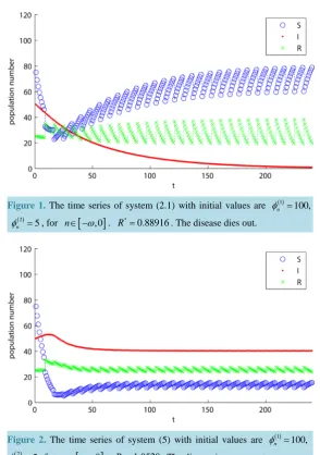
[image:13.595.178.451.119.241.2] [image:13.595.165.460.286.705.2]

Let

β

=0.18, then R*=0.88916<1. According to Theorem 4, we know that the disease will die out (see Figure 1). Let

β

=0.214, then R*=1.0529>1. According to Theorem 5, we know that the disease will be permanent (see Figure 2).

Figure 1. The time series of system (2.1) with initial values are φn( )1 =100,

( )2

5

n

φ = , for n∈ −

[

ω,0

]

. R*=0.88916. The disease dies out.

Figure 2. The time series of system (5) with initial values are ( )1

100,

n

φ =

( )2

5

n

(14)

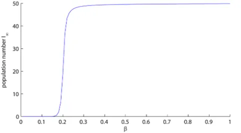
Figure 3 shows a bifurcation diagram for stroboscopic map of system (2.1) with the infection rate

β

as the bifurcation parameter. This is illustrated in Figure 4 by the curve

I

_∞ (the number of infection individuals at the equilibrium) that varies with

β

. We can observe that the value of

I

_∞ increases as

β

increases, and

I

_∞ is hypersensitive when β∈

(

0.2, 0.215

)

, or else it is insensitive.

[image:14.595.197.438.193.326.2]

Figure 4 shows a bifurcation diagram for stroboscopic map system (2.1) with pulse vaccination rate θ as the bifurcation parameter (for which R_* >1). In this case, numerical result implies that there is unique positive equilibrium of stroboscopic map for all θ, that is, there is a positive periodic solution of system (2.1) for all θ. As Figure 5 and Figure 6 shown, it can be seen that the positive equilibrium is globally attractive.

[image:14.595.196.442.371.507.2]

Figure 3. The bifurcation diagram the unique endemic equilibrium (the com- ponent I of infectious individuals regarding β as the bifurcation parameter, all other parameters are same as in model (5.1)).

Figure 4. The bifurcation diagram the unique endemic equilibrium (the com- ponent I of infectious individuals regarding θ as the bifurcation parameter, all other parameters are same as in model (5.1) except for β =0.214).

(a) (b)

[image:14.595.102.538.556.704.2]

(15)

[image:15.595.171.462.86.240.2] [image:15.595.169.459.262.445.2]

Figure 6. The phase diagram of system (2.1). R_*=1.0529.

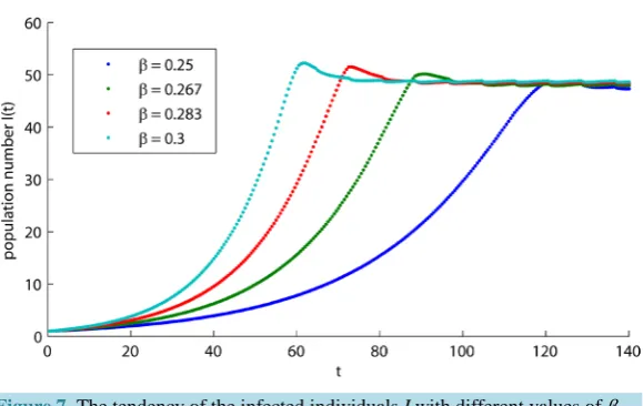
Figure 7. The tendency of the infected individuals I with different values of β.

Therefore, an interesting open problem is proposed whether we can prove that the positive periodic solution of model (2.1) is globally attractive as

R

_*

>

1

.

Finally, the numerical simulations of the stroboscopic map of model on the number of infected individuals with different values of

β

are shown in Figure 7. It shows that the number of infected individuals will in- crease steadily in next few days, then reach the peak and begin a slow decline, and finally become stable. The greater the value

β

, the bigger the peak value and the earlier the peak appears. Our result implies that decreasing infection rate can put off the disease outbreak and reduce the number of infected individuals.

Acknowledgements

The research has been supported by the Natural Science Foundation of China (11261004, 11561004), the Sci- ence and Technology Plan Projects of Jiangxi Provincial Education Department (GJJ14673) and the Social Sci- ence Planning Projects of Jiangxi Province (14XW08).

References

[1] Agur, Z., Cojocaru, L., Mazor, G., et al. (1993) Pulse Mass Measles Vaccination across Age Cohorts. Proceedings of

the National Academy of Sciences of the United States of America, 90, 11698-11702.

http://dx.doi.org/10.1073/pnas.90.24.11698

[2] Beretta, E. and Takeuchi, Y. (1995) Global Stability of an SIR Epidemic Model with Time Delays. Journal of

Mathe-matical Biology, 33, 250-260. http://dx.doi.org/10.1007/bf00169563

(16)

http://dx.doi.org/10.1016/S0362-546X(01)00528-4

[4] Takeuchi, Y., Ma, W. and Beretta, E. (2000) Global Asymptotic Properties of a Delay SIR Epidemic Model with Finite Incubation Times. Nonlinear Analysis: Theory, Methods & Applications, 42, 931-947.

http://dx.doi.org/10.1016/S0362-546X(99)00138-8

[5] Ma, W., Song, M. and Takeuchi, Y. (2004) Global Stability of an SIR Epidemic Model with Time Delay. Applied

Ma-thematics Letters, 17, 1141-1145. http://dx.doi.org/10.1016/j.aml.2003.11.005

[6] Song, M., Ma, W. and Takeuchi, Y. (2007) Permanence of a Delayed SIR Epidemic Model with Density Dependent Birth Rate. Journal of Computational and Applied Mathematics, 201, 389-394.

http://dx.doi.org/10.1016/j.cam.2005.12.039

[7] Cooke, K.L. (1979) Stability Analysis for a Vector Disease Model. Rocky Mountain Journal of Mathematics, 9, 31-42. http://dx.doi.org/10.1216/RMJ-1979-9-1-31

[8] Zhang, B. and Liu, Y. (2003) Global Attractivity for Certain Impulsive Delay Differential Equations. Nonlinear

Analy-sis: Theory, Methods & Applications, 52, 725-736. http://dx.doi.org/10.1016/S0362-546X(02)00129-3

[9] Du, Y. and Xu, R. (2010) A Delayed SIR Epidemic Model with Nonlinear Incidence Rate and Pulse Vaccination.

Journal of Applied Mathematics & Informatics, 1089-1099.

[10] Yan, J., Zhao, A. and Nieto, J.J. (2004) Existence and Global Attractivity of Positive Periodic Solution of Periodic Single-Species Impulsive Lotka-Volterra Systems. Mathematical and Computer Modelling, 40, 509-518.

http://dx.doi.org/10.1016/j.mcm.2003.12.011

[11] Zhang, X.B., Huo, H.F., Sun, X.K., et al. (2010) The Differential Susceptibility SIR Epidemic Model with Time Delay and Pulse Vaccination. Journal of Applied Mathematics and Computing, 34, 287-298.

http://dx.doi.org/10.1007/s12190-009-0321-y

[12] Capasso, V. and Serio, G. (1978) A Generalization of the Kermack-Mckendrick Deterministic Epidemic Model.

Ma-thematical Biosciences, 42, 43-61. http://dx.doi.org/10.1016/0025-5564(78)90006-8

[13] Lambert, J.D. (1991) Numerical Methods for Ordinary Differential Systems: The Initial Value Problem.

[14] Sekiguchi, M. and Ishiwata, E. (2011) Dynamics of a Discretized SIR Epidemic Model with Pulse Vaccination and Time Delay. Journal of Computational and Applied Mathematics, 236, 997-1008.

http://dx.doi.org/10.1016/j.cam.2011.05.040

[15] Mickens, R.E. (1999) Discretizations of Nonlinear Differential Equations Using Explicit Nonstandard Methods.

Jour-nal of ComputatioJour-nal and Applied Mathematics, 110, 181-185. http://dx.doi.org/10.1016/S0377-0427(99)00233-2

[16] Piyawong, W., Twizell, E.H. and Gumel, A.B. (2003) An Unconditionally Convergent Finite-Difference Scheme for the SIR Model. Applied Mathematics and Computation, 146, 611-625.

http://dx.doi.org/10.1016/S0096-3003(02)00607-0

[17] Jódar, L., Villanueva, R.J., Arenas, A.J., et al. (2008) Nonstandard Numerical Methods for a Mathematical Model for Influenza Disease. Mathematics and Computers in Simulation, 79, 622-633.

http://dx.doi.org/10.1016/j.matcom.2008.04.008

[18] Erjaee, G.H. and Dannan, F.M. (2004) Stability Analysis of Periodic Solutions to the Nonstandard Discretized Model of the Lotka-Volterra Predator-Prey System. International Journal of Bifurcation and Chaos in Applied Sciences and

Engineering, 14, 4301-4308. http://dx.doi.org/10.1142/S0218127404011946

[19] Solis, F.J. and Chen-Charpentier, B. (2004) Nonstandard Discrete Approximations Preserving Stability Properties of Continuous Mathematical Models. Mathematical and Computer Modelling, 40, 481-490.

http://dx.doi.org/10.1016/j.mcm.2004.02.028

[20] Su, H. and Ding, X. (2008) Dynamics of a Nonstandard Finite-Difference Scheme for Mackey-Glass System. Journal

of Mathematical Analysis and Applications, 344, 932-941. http://dx.doi.org/10.1016/j.jmaa.2008.03.044

[21] Roeger, L.-I.W. (2008) Dynamically Consistent Discrete Lotka-Volterra Competition Models Derived from Nonstan-dard Finite-Difference Schemes. Discrete and Continuous Dynamical Systems—Series B, 9, 415-429.

http://dx.doi.org/10.3934/dcdsb.2008.9.415

[22] Ma, W., Takeuchi, Y., Hara, T., et al. (2002) Permanence of an SIR Epidemic Model with Distributed Time Delays.