Optimal forecasting model selection and data characteristics

Munich Personal RePEc Archive

Optimal forecasting model selection and

data characteristics

Fildes, Robert and Madden, Gary and Tan, Joachim

Lancaster University, Lancaster University Management School, UK,

Curtin University of Technology, Perth, Australia, Curtin University

of Technology, Perth, Australia

2007

Online at

https://mpra.ub.uni-muenchen.de/10819/

PLEASE SCROLL DOWN FOR ARTICLE

On: 26 September 2008

Access details: Access Details: [subscription number 788741507] Publisher Routledge

Informa Ltd Registered in England and Wales Registered Number: 1072954 Registered office: Mortimer House, 37-41 Mortimer Street, London W1T 3JH, UK

Applied Financial Economics

Publication details, including instructions for authors and subscription information:

http://www.informaworld.com/smpp/title~content=t713684415

Optimal forecasting model selection and data characteristics

a _{Lancaster University, Lancaster, LA1 4YX, UK} b _{Curtin University of Technology, School of Economics and} Finance, Perth, WA 6845, Australia c _{Curtin University of Technology, Perth, WA 6845, Australia}

First Published on: 02 May 2007

To cite this Article Fildes, Robert, Madden, Gary and Tan, Joachim(2007)'Optimal forecasting model selection and data characteristics',Applied Financial Economics,17:15,1251 — 1264

To link to this Article: DOI: 10.1080/09603100600905061 URL: http://dx.doi.org/10.1080/09603100600905061

Full terms and conditions of use: http://www.informaworld.com/terms-and-conditions-of-access.pdf

This article may be used for research, teaching and private study purposes. Any substantial or systematic reproduction, re-distribution, re-selling, loan or sub-licensing, systematic supply or distribution in any form to anyone is expressly forbidden.

Optimal forecasting model selection

and data characteristics

Robert Fildes

, Gary Madden

* and Joachim Tan

a

Lancaster University, Lancaster University Management School, Lancaster, LA1 4YX, UK

b

Curtin University of Technology, School of Economics and Finance, GPO Box U1987, Perth, WA 6845, Australia

c

Curtin University of Technology, School of Economics and Finance, Perth, WA 6845, Australia

Selection protocols such as Box–Jenkins, variance analysis, method switching and rules-based forecasting measure data characteristics and incorporate them in models to generate best forecasts. These protocol selection methods are judgemental in application and often select a single (aggregate) model to forecast a collection of series. An alternative is to apply individually selected models for to series. A multinomial logit (MNL) approach is developed and tested on Information and commu-nication technology share price data. The results suggest the MNL model has the potential to predict the best forecast method based on measurable data characteristics.

I. Introduction

Selection protocols such as Box–Jenkins, variance analysis (Gardner and McKenzie, 1988), method switching (Goodrich, 1990), Automatic Identification (Vokurka et al., 1996) and rules-based forecasting (Collopy and Armstrong, 1992; Adya et al., 2001) measure data characteristics and incorporate them in models to generate best forecasts. These protocol selection methods are judgemental in their applica-tion and often select a single (aggregate) model to forecast a collection of series. Fildes (1989) suggests there are gains to be made in forecast accuracy when applying individually selected models by series. Shah (1997) applies discriminant analysis to select the best forecasting model based on the discriminant scores of data characteristics and demonstrates that an individual selection approach provides more accurate forecasts than an aggregate selected model. In this study, an alternative individual selection approach

is developed using a multinomial logit (MNL) approach to relate data characteristics to out-of-sample forecast accuracy. The results, applied to information and communication technology (ICT) share price data, suggests the MNL model has the potential to predict the best forecast method based on measurable data characteristics. In particular, the MNL-based procedure is trialled on ICT share price data for recent Growth-to-Bust (January 1993 to March 2000) and Bust-to-Recovery (October 2001 to December 2002) phases, and for the periods combined.

II. Model Selection Using the Multinomial Logit Model

The application of the MNL model to individually select a forecast model for a series assumes the

*Corresponding author. E-mail: [email protected]

Applied Financial EconomicsISSN 0960–3107 print/ISSN 1466–4305 onlineß2007 Taylor & Francis 1251 http://www.tandf.co.uk/journals

DOI: 10.1080/09603100600905061

post-sample forecast accuracy of a forecasting method is a function of measurable sample char-acteristics that are sufficient in describing a series. It also implies a sampled series is well forecast by one of the models applied to these data.1 To develop selection rules using the MNL approach, an optimal forecast method from a selection of methods for a series is first determined based on a minimum error criterion. This is done by omitting a set of observa-tions from the estimation period and selecting the method that generates the highest accuracy in one-step ahead forecasts for all the omitted observations. Next, the MNL model is estimated to statistically identify any relationships that exist between the best forecast method, data moments and time-series characteristics. Best forecast model probabilities are then calculated and compared against the best forecast methods.

The MNL model is specified as:

PðYi¼jÞ ¼

ez0

itj

PJ

m¼1ez

0

itm, j¼1,

. . ._{,J ð1Þ}

whereziis a vector of data series characteristics and

j indexes associated forecast methods. The MNL approach is useful as it allows the estimation of conditional probabilities that relate the success of a forecasting model of a series, Yi, based on collected

data characteristics for the series zi. From the

conditional probabilities, forecasts are generated for methods with the greatest posterior probability and compared against the individual forecasting method that generates the lowest error for comparison.

III. Forecasting Models

The forecasting methods employed for the analysis are exponential smoothing and ARMA-based models, viz., the ARARMA, ARIMA, Holt, Holt-D, Holt-Winters, Robust Trend and simple exponential smoothing (SES). These models are chosen as they consistently perform well in the M-competition of Makridakis et al. (1993) and

Makridakis and Hibon (2000). Exponential smooth-ing models assume a series comprises of a systematic and a random variation that can be described by level and trend (Meade, 2000). The corresponding smooth-ing methods considered are Holt, D, Holt-Winters (Holt-W) and simple exponential smooth-ing.2 As an alternative approach, Grambsch and Stahel’s (1990) robust trend (RT), a nonparametric version of a linear trend, is also estimated. RT provides a good base for comparison because it is median-based model that is not sensitive to outliers. The ARMA-based models that are applied are ARARMA and ARIMA (p,d,q). Parzen’s (1982) ARARMA model is a long-memory method that uses a best fit AR model, according to the least Akaike information criterion (AIC) statistic, as a filter to difference series prior to estimating the best fitting ARMA model (also selected by the AIC statistic).3 The ARIMA (p,d,q) model is chosen as it is suitable for nonstationary share prices. Adopting this ARIMA model specification assumes share prices are not seasonally influenced or affected by other factors.4

To select a best fit ARIMA (p,d,q) model for estimation the Meade (2000) procedure is applied. First, the number of differences required to render a series stationary is determined by applying the Geweke and Porter-Hudek (GPH; 1983) method. The GPH method is useful as it estimates the number of differences as a real number for the autoregressive fractionally integrated moving average model and can be used as an approximation to estimate the number of differences for the ARIMA. As ARIMA requires differencing to be an integer, the estimated GPH value for a series is converted to an integer by the rule, when d< 0.5 then d¼0, otherwise d¼integer part of dþ0.5. After differencing, alternative ARIMA models are estimated by series via a grid search of up to 7 lags generating 49 ARIMA models per differenced series.5From the estimated ARIMA models a best fitting model is chosen by the least AIC statistic. Estimation for a series begins at observation 10 to allow a maximum seven period lag estimate for the ARIMA and ARARMA models. Forecasts are

1

A series is regarded as ‘belonging to a method’ if that method generates the lowest out-of-sample forecast errors. However, this does not imply the associated model is the data generating process for the series.

2

Holt-D is a deseasonalized Holt model. A thorough description of other exponential smoothing models is given by Gardner and McKenzie (1988).

3

While Parzen (1982) uses an autoregressive transfer function (CAT) criterion to select a best AR filter he notes the selection of the filter by the CAT and AIC are similar.

4

In this situation, seasonal ARIMA or ARMAX models could be applied.

5

A grid search estimates all possible lag combinations of ARIMA(p,d,q) and selects the best fitting model based on an error statistic.

1252

R. Fildes

et al.

then generated for best models by method. Holt, Holt-D, Holt-W, RT and SES models have a fixed lag length and do not require grid searches to select the best model.6The grid search for an optimal lag length for the ARARMA and ARIMA models are based on the least AIC statistic.

IV. Forecast Error Measures

Selection of best forecast model is based on the geometric root mean squared error (GRMSE; Fildes, 1992) and root mean squared error (RMSE) forecast error statistics. Fildes and Ord (2002) argue the GRMSE is the preferable measure as it is unaffected by scale change. Also, Armstrong and Collopy (1992) consider the GRMSE is the more reliable as it is sensitive to small changes but unaffected by outliers. The RMSE statistic is calculated to provide a basis for comparison. To estimate the GRMSE and RMSE for each series and method, theh-step ahead forecast error "i,T,j(h) made in forecasting period Tþh for

series ifor methodjis calculated as,

"i,T,jðhÞ ¼ Ai,Tþh,jFi,T,jðhÞ

whereTis the end point of the estimation period and forecast origin,Fi,T,j(h) is theh-step forecast for series

i and method j and Ai,Tþh,j is the actual value at

periodTþhfor seriesi. From the forecast error, the

h-step mean squared error MSEi,T,j(h) for series i

and methodjis,

MSEi,T,jðhÞ ¼

1

n X

"i,Tþh,j

2

wherenis the length of the forecast period beginning with Tþ1. The h-step root mean squared error

RMSEi,T,j(h) for seriesiand methodjis,

RMSEi,T,jðhÞ ¼

ffiffiffiffiffiffiffiffiffiffiffiffiffiffiffiffiffiffiffiffiffiffiffiffi MSEi,T,jðhÞ p

:

The scale-invariant h-step GRMSE error statistic

GRMSEi,T,j(h) for seriesiand method jis,

GRMSEi,T,jðhÞ ¼

Yn 1

"2_i,t,j

!1=2n

V. ICT Industry Share Price Data

ICT industry share prices experienced substantial volatility from 1994 to 2002. From 1994 to 2000, deregulation of global ICT markets ushered in an industry-wide boom (1 January 1994 to 6 March 2000). However, the ‘dot.com’ bubble burst due to an overly rapid rate of infrastructure investment. This investment created an excess supply of productive capacity, relative to demand growth, that led to a spectacular collapse in stock prices from 10 March 2000 to 30 September 2001 (Cooper and Madden, 2004). It is estimated that approximately US$ 2 trillion of market value for these companies was lost as a result of the bursting of the ICT bubble (Hausman, 2004). While the ICT industry has managed a sustained period of slow recovery (1 October 2001 to 31 December 2002) it seems unlikely these companies will revisit the high valua-tions of the boom period. Accordingly, this volatile period presents an ideal opportunity to test whether the MNL-based protocol can guide the making of better forecasts for historical ICT share price series.

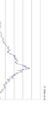
The share price sample is separated into distinct Boom (1 January 1994 to 9 March 2000—1616 observations), Bust (10 March 2000 to 3 October 2001—666 observations), Combined (1 January 1994 to 3 October 2001) and Recovery (4 October 2001 to 31 December 2002—320 observations) phases (Fig. 1). These data are acquired from DataStream International and consist of 108 United States (US) ICT company share market prices from 1 January 1994 to 31 December 2002 (2610 observations).7 A representative specimen of these data is shown in Fig. 2. The shares prices are daily closing share prices denominated in US dollars (US$).

Figure 2 suggests these data exhibit characteristics typical of a nonstationary time series (which is a feature common of share prices). Nonstationarity is often caused by a tendency for share prices to experience positive drift. When applying a model to nonstationary data a common econometric practice is to first-difference the series prior to model estimation. Differencing renders an AR1 series stationary. However, the method also removes features of these data, such as drift, that may assist in obtaining accurate forecasts. An alternative procedure that

6

Linear, no-trend and nonseasonal Holt, and Holt-W models are considered. Parameters are estimated and not fixed arbitrarily.

7

These data consist only of share prices for ICT companies that survived the sample period. Hence, the study results may exhibit survivorship bias.

0

100 200 300 400 500 600

31/12/1993 31/03/1994 30/06/1994 30/09/1994 31/12/1994 31/03/1995 30/06/1995 30/09/1995 31/12/1995 31/03/1996 30/06/1996 30/09/1996 31/12/1996 31/03/1997 30/06/1997 30/09/1997 31/12/1997 31/03/1998 30/06/1998 30/09/1998 31/12/1998 31/03/1999 30/06/1999 30/09/1999 31/12/1999 31/03/2000 30/06/2000 30/09/2000 31/12/2000 31/03/2001 30/06/2001 30/09/2001 31/12/2001 31/03/2002 30/06/2002 30/09/2002 Fig. 1. FTSE world telecom service index, January 1994–December 2002 Source : Thomson Financial (2004).

0 10 20 30 40 50 60 70 80 90

100 3/01/1994 3/04/1994 3/07/1994 3/10/1994 3/01/1995 3/04/1995 3/07/1995 3/10/1995 3/01/1996 3/04/1996 3/07/1996 3/10/1996 3/01/1997 3/04/1997 3/07/1997 3/10/1997 3/01/1998 3/04/1998 3/07/1998 3/10/1998 3/01/1999 3/04/1999 3/07/1999 3/10/1999 3/01/2000 3/04/2000 3/07/2000 3/10/2000 3/01/2001 3/04/2001 3/07/2001 3/10/2001 3/01/2002 3/04/2002 3/07/2002 3/10/2002 Fig. 2. Time warner share price series, January 1993–December 2002 Source : Thomson Financial (2004).

1254

R.

Fildes

et

al.

might be considered is the incorporation of series characteristics into modeling the data generating process. For this study, series characteristics are collected and used to determine which of these characteristics are helpful in determining the best forecasting model via a MNL model. Data charac-teristics collected for this purpose are series moments (mean, variance, skewness and kurtosis) and selected time-series characteristics (coefficient of variation, number of outliers, step changes, turning points, trend direction, extreme last observations and ARCH effects).

To enable MNL model estimation, data on series characteristics are collected. Of the characteristics described by Collopy and Armstrong (1992), Shah (1997), Fildes et al. (1998) and Meade (2000), the mean, median, variance, skewness, kurtosis, step changes, turning points, number of outliers, coeffi-cient of variation, presence of ARCH effects, trend direction and the presence of an extreme last observation are calculated.8 Outliers are defined as observations that exceed 3 SDs of a series mean. Step changes and turning points are as defined by Shah (1997). A turning point captures oscillating behaviour by a seriesXtwhile a step change identifies structural

breaks in a series. That is, a turning point is any observation contained in a series (1 <t<T) for which

Xt1<XtandXtþ1<XtorXt1>XtandXtþ1>Xt.

A step change occurs in a series when the absolute difference of an observation and its lagged meanXt1

exceed twice the lagged SD of the seriesSt1, viz.,

XtXt1

>2st1, t¼1,. . .,T

A series with a relatively large number of structural breaks will exhibit relatively many step changes. Trend direction and the presence of an extreme last observation are as defined by Meade (2000). Trend direction is a binary variable that determines whether the basic and recent trend of a series is similar in direction. The basic trend is the gradient of the regression of a series against time containing all observations, while the recent trend is the gradient of a similar regression performed with only the last six observations. The trend variable value equals unity when the basic and recent trend of a series is in the same direction and zero otherwise. An extreme last observation is any last observation that is greater than 90% of the largest observation,

XT> 0.9Max(X1,. . .,XT1), or is less than 110% of the smallest observation,

XT> 1.1 Min(X1,. . .,XT1). Hence, this variable has the value unity is the presence of an extreme last observation and zero otherwise. The variable for the presence of an ARCH effect is a binary variable that is determined by the result of Engle’s (1982) Lagrange multiplier (LM) test with a one-period lag. The variable has the value unity when an ARCH effect is detected by the LM test and zero otherwise. The LM test for ARCH is applied to the residuals of the best fitting ARIMA model determined by the lowest AIC.

VI. Best Forecast Model

To determine the best forecast model for a series the post-sample performance of the seven forecast

Re-estimation

Model selection

Estimation Forecast

Estimation Model selection Forecast Step 1

Step 2

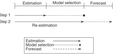
Fig. 3. MNL estimation and forecast procedure

Note: The procedure is applied to the Boom Phase (1 January 1994 to 9 March 2000); Bust Phase (10 March 2000 to 3 October 2001); and Combined Phase (1 January 1994 to 3 October 2001).

8

Other data characteristics described by these studies are not collected as they either describe similar series features or are highly correlated other characteristics.

models are related to in-sample series characteristics via an MNL model. To do so a dependent polychotomous variable is generated that indicates best series forecast method based on an error statistic.

That is, the variable has the value unity for the best forecast method that generates the lowest errors and a zero for the remaining six forecast methods. However, only the results based on the GRMSE

Table 1. Boom phase data characteristic summary—108 series

Mean SD Skewness Kurtosis Minimum Maximum Mean 0.0009 0.0007 0.7466 4.5320 0.0007 0.0034 Variance 0.0008 0.0005 0.5760 2.7088 0.0001 0.0025 Skewness 0.4085 0.8829 0.2059 2.8901 1.7648 2.4452 Kurtosis 13.3092 34.6624 5.3303 31.7958 0.9420 245.6450 Outliers 20.1111 4.7426 0.4638 3.4609 10.0000 35.0000 Step change 0.0486 0.0068 0.6695 4.2114 0.0248 0.0652 Turn point 0.6344 0.0453 7.4384 66.9699 0.2191 0.6760

Runs 1047 57 8 77 502 1102

Notes: SD is the standard deviation; Step change is the ratio of step changes to number of observations; Turn point is the ratio

of turning points to number of observations and Outliers is ratio of outliers that are larger than 3 SDs to the number of observations. The presence of ARCH is detected by fitting the most appropriate ARIMA model (lowest AIC) and tests for the prescience of ARCH in the residuals. The sample proportion with an ARCH effect is 95.37%.

Table 2. Bust phase data characteristic summary—108 series

Mean SD Skewness Kurtosis Minimum Maximum Mean 0.0002 0.0009 0.1153 3.4598 0.0030 0.0022 Variance 0.0016 0.0011 1.3015 6.8954 0.0002 0.0071 Skewness 0.1926 0.8054 0.0129 3.0058 2.0570 2.1919 Kurtosis 8.1359 13.1480 3.2204 13.7959 0.2301 72.4225 Outliers 7.5741 2.4350 0.3722 2.9838 3.0000 15.0000 Step change 0.0481 0.0089 0.7854 3.2918 0.0210 0.0615 Turn point 0.6544 0.0267 3.9244 31.0762 0.4528 0.6987

Runs 440 14 2 11 359 467

Notes: SD is the Standard deviation; Step change is the ratio of step changes to number of observations; Turn point is the

ratio of turning points to number of observations and Outliers is ratio of outliers that are larger than 3 SDs to the number of observations. The presence of ARCH is detected by fitting the most appropriate ARIMA model (lowest AIC) and tests for the prescience of ARCH in the residuals. The sample proportion with an ARCH effect is 50.93%.

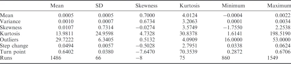
Table 3. Boom and Bust data characteristic summary—108 series

Mean SD Skewness Kurtosis Minimum Maximum Mean 0.0005 0.0005 0.7000 4.0124 0.0004 0.0022 Variance 0.0010 0.0007 0.6734 3.2063 0.0001 0.0034 Skewness 0.0107 0.7314 0.0274 3.5749 1.7550 2.2538 Kurtosis 13.9811 24.9598 4.7328 30.8378 1.6141 198.5190 Outliers 29.7222 6.3405 0.5132 4.0909 16.0000 53.0000 Step change 0.0494 0.0057 0.5028 2.7951 0.0338 0.0624 Turn point 0.6402 0.0380 7.6470 70.3539 0.2872 0.6706

Runs 1486 66 8 75 860 1549

Notes: SD is the standard deviation; Step change is the ratio of step changes to number of observations; Turn point is the ratio

of turning points to number of observations and Outliers is ratio of outliers that are larger than 3 SDs to the number of observations. The presence of ARCH is detected by fitting the most appropriate ARIMA model (lowest AIC) and tests for the prescience of ARCH in the residuals. The sample proportion with an ARCH effect is 85.19%.

1256

R. Fildes

et al.

are reported. MNL models are estimated for the Boom phase, Bust phase and a Boom and Bust (Combined) period based on the raw stock price data. This procedure is followed to allow for the possibility that the structural relationship between the best forecasting method and series characteristics may change. MNL model estimation is intended to indicate the importance of series characteristics in determining best forecast method. That is, the protocol potentially relates series data typology to best forecast method.

From the seven models, sample forecasts are generated. Figure 3 illustrates the MNL procedure applied to the Bust, Recovery and Combined phases. The best fit model is selected on the basis of out-of-sample forecast accuracy for the Bust, Recovery and Combined phases. To forecast out-of-sample, all observations other than the last 22 of the Boom, Bust and Combined phases are used for estimating the forecasting models.9 The estimated models are then used to forecast the last 22 observations for a phase. Based on forecasts generated from the models by phase, a best fit model is chosen. The choice is made by comparing the forecast errors of the last 22 observations according to an error statistic and selecting the model that generates the lowest error by phase. The best fit models by phase are then re-estimated for the entire phase and forecasts are generated for the subsequent phase. The first forecast period focuses on forecasting the 666 Bust phase observations, while the second and third periods focuses on the remaining 320 observations in the Recovery phase.

VII. Sample Data Characteristics

Tables 1–3 present the summary statistics of the 108 returns series contained in the sample by phase, respectively.

In the Boom phase, share prices experienced frequent rises with market valuations typically increasing through the period. Many firms consis-tently experienced ‘new’ high prices. Table 1 presents share price returns sample statistics for the 108 series for the Boom phase. Consistent with increasing share prices, the returns are on an average positive, positively skewed and contain many outliers. The

statistics also reveal 5% of the series contain step changes and95% of series record an ARCH effect. This outcome implies the increasing risk shares faced over the Boom phase.

Inspection of the statistics for the share price returns contained in Table 2 for the Bust phase show a distinctly different picture to that of the Boom phase. The Bust phase is characterized by falling share prices after the bursting of the dot.com bubble. The negative mean and negative skewness of returns clearly illustrates this phenomenon. Other notable differences from the Boom phase are that the series generally exhibit a higher variance, less kurtosis, fewer outliers and runs. Also there is a lower percentage of series (51%) recording an ARCH effect. The proportion of step changes and turning points to observations remain unchanged for the sample across the Boom and Bust phases.

Table 3 reports the sample statistics for the combined Boom and Bust phases. As might be expected, the statistics show average returns have a positive mean and are positively skewed. This out-come results from the Boom period being twice as long as that for the Bust period. Table 3 also reports more outliers and runs for the combined period. Further, the combined sample shows a relatively high incidence of ARCH effects.

VIII. Results

Boom phase MNL estimation

GRMSE results reported in Table 4 show the Holt-D is the better forecast method, relative to SES, based on these series characteristics. Holt-D is more likely the better method forecast the larger is the mean, skewness, kurtosis and coefficient of variation values, and when ARCH, step changes and turning points are present. Holt-D is less preferred when the series variance and number of outliers is higher, and when an extreme last observation occurs. The Holt model is preferred when the series has fewer outliers and runs with no extreme last observation, and when an ARCH effect is detected. The ARIMA model forecasts better, relative to SES, the lower is the value of the skewness.10 The results reported in Table 5 show that the MNL model based on estimated GRMSE values is effective in selecting

9

Twenty-two observations are chosen to represent a 30-day month with five weekly trading days.

10

The trend variable is not included in the MNL estimation for this period due to a strong negative correlation with sample kurtosis values.

Table 4. Boom phase MNL model estimates based on GRMSE

Model Mean Variance Skewness Kurtosis Step chg Turn point Outlier Runs CV ARCH Extreme

ARARMA 0.07 (0.07) 0.17 (0.23) 0.01 (0.01) 0.20 (0.27) 10.50 (26.17) 6.67 (16.01) 1.64 (1.94) 0.01 (0.01) 0.16 (2.62) 1.38 (2.41) 0.78 (0.69)

ARIMA 0.24 (0.17) 0.69 (0.53) 0.05* (0.02) 0.13 (0.46) 50.70 (51.97) 14.81 (22.03) 6.86 (5.24) 0.02 (0.01) 7.34 (4.96) 2.61 (2.89) 1.30 (1.04)

Holt 0.09 (0.11) 0.18 (0.13) 0.03 (0.03) 0.78 (0.69) 21.86 (42.44) 39.11 (28.72) 11.80* (4.60) 0.07* (0.03) 7.39 (5.63) 44.06* (18.18) 45.25* (9.13)

Holt-D 2.78* (1.22) 8.39* (3.71) 0.50* (0.23) 2.53* (0.98) 870.33* (396.18) 891.52* (408.67) 65.17* (27.40) 0.61* (0.29) 70.81 (33.98) 21.44 (21.26) 16.95* (7.25)

Holt-W 0.07 (0.06) 0.17 (0.19) 0.02 (0.02) 0.14 (0.33) 8.47 (31.85) 15.20 (17.95) 0.38 (2.03) 0.01 (0.01) 2.30 (3.23) 3.83 (2.02) 0.35 (1.06)

RT 0.00 (0.02) 0.01 (0.03) 0.01 (0.02) 0.06 (0.33) 1.96 (34.05) 6.28 (12.99) 1.09 (1.86) 0.00 (0.01) 1.11 (2.73) 1.08 (1.72) 1.16 (0.94)

Notes: SD is the standard deviation. Step change and Turn point are the step changes and turning points divided by the number of observations; Outlier is outliers larger than 3 SDs; CV is the coefficient of variation; ARCH and Trend are binary variables; where¼1 in the presence of an ARCH effect and¼0 otherwise and¼1 when the basic trend is in the same direction as the recent trend (over the last 30 days), respectively. ARCH tests are performed by fitting the most appropriate ARIMA model (lowest AIC) and testing for the presence of ARCH in the residuals. The likelihood ratio R2 for this model (against a model with a constant only) is 0.191. SDs are in parenthesis. * is significant at the 5% level.

1258

R.

Fildes

et

al.

the better forecasting model in the Boom phase. The MNL model based on the GRMSE is able to correctly indicate the best model in 57.4% of the 108 series. In particular, MNL model correctly predicts the ARARMA and Holt-D models in 94.7% and 50.0% of the cases, respectively. However, the MNL model is unable to correctly select the ARIMA, Holt, Holt-W, RT and SES models when they perform best.11

Bust phase MNL estimation

The GRMSE results reported in Table 6 are, not surprisingly, less definitive given the Bust period share price turbulence.12 ARIMA forecasts better, relative to the SES when an extreme last observation occurs. The Holt model performs better when there is no series trend and no extreme last observation occurs. Holt-D’s performance is better, relative to the SES, the greater is the kurtosis value, number of turning points and when the series contains an extreme last observation. Holt-D is not preferred to

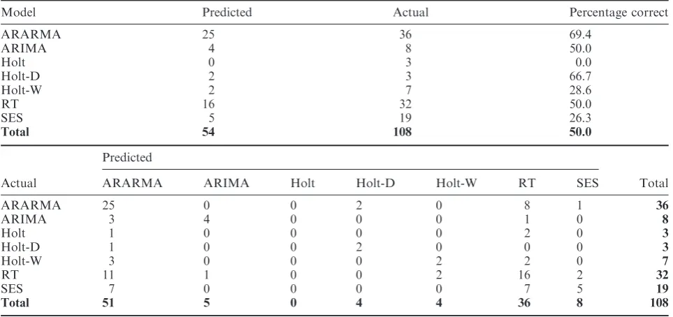
the SES when there is a large number of step changes and outliers in the sample. Holt-W is better when there is a series trend and no extreme last observation arises. The results contained in Table 7 for the MNL model based on estimated GRMSE in the Bust phase results are qualitatively dissimilar to those reported for the Boom phase. The MNL model is not as effective in indicating the better forecasting model for the Bust phase. The model correctly indicates the best model for 50.0% of the 108 series in the Bust phase compared to 57.4% in the Boom phase. Also, Table 7 show the MNL model correctly indicates the ARARMA, ARIMA, Holt-D and RT models in 69.4%, 50%, 66.7% and 50.0% of cases, respectively. However, the MNL model is unable to correctly select the Holt, Holt-W and SES models.13

Combined period MNL estimation

The MNL model based on the GRMSE for the combined Boom and Bust phases are reported in Tables 8 and 9.14The tables indicate that Holt-D and

Table 5. Boom phase predictions based on GRMSE

Model Predicted Actual Percentage correct

ARARMA 54 57 94.7

ARIMA 0 4 0.0

Holt 1 6 16.7

Holt-D 1 2 50.0

Holt-W 3 13 23.0

RT 3 13 23.0

SES 0 13 0.0

Total 62 108 57.4

Predicted

Actual ARARMA ARIMA Holt Holt-D Holt-W RT SES Total

ARARMA 54 0 0 0 2 1 0 57

ARIMA 4 0 0 0 0 0 0 4

Holt 5 0 0 1 0 0 0 6

Holt-D 0 0 1 1 0 0 0 2

Holt-W 10 0 0 0 3 0 0 13

RT 10 0 0 0 0 3 0 13

SES 12 0 0 1 0 0 0 13

Total 95 0 1 3 5 4 0 108

11

The MNL results based on the RMSE show the model correctly indicates the best model in 57.4% of the 108 cases. The MNL indicates ARARMA model correctly in 94.8% of cases. However, the model is unable to correctly indicate the ARIMA, Holt, Holt-D, Holt-W, RT and SES models. Results are available on request.

12

In Bust phase MNL model estimation, the number of runs is excluded due to a high positive correlation with the number of turning points.

13

The MNL model based on the RMSE correctly indicates the better model in 44.4% of the 108 series. The model correctly indicates the ARARMA, Holt-D and RT models in 69.4%, 50.0% and 58.6% of cases, respectively. However, the model is unable to correctly indicate the ARIMA, Holt, Holt-W and SES models. Results are available on request.

14

In combined phase, the coefficient of variation and extreme variable is omitted from the MNL estimation due to strong positive correlation with skewness values.

Table 6. Bust phase MNL model estimates based on GRMSE

Model Mean Variance Skewness Kurtosis Step chg Turn point Outlier CV ARCH Extreme Trend

ARARMA 0.01 (0.03) 0.01 (0.11) 0.02 (0.02) 0.04 (1.01) 3.31 (34.05) 2.61 (6.51) 2.86 (1.96) 0.45 (6.78 0.09 (0.70) 0.69 (0.73) 0.62 (0.68)

ARIMA 0.04 (0.09) 0.07 (0.24) 0.06 (0.04) 0.89 (1.43) 87.71 (53.57) 4.83 (9.59) 0.52 (3.38) 2.18 (10.40) 0.83 (1.26) 4.33* (1.47) 0.37 (1.19)

Holt 0.08 (0.07) 0.12 (0.24) 0.00 (0.03) 0.68 (4.71) 1.97 (97.61) 5.69 (12.55) 0.01 (3.49) 7.24 (15.56) 0.82 (1.33) 27.97* (1.05) 29.09* (1.02)

Holt-D 0.16 (0.37) 0.77 (1.63) 0.28 (0.18) 13.01* (5.44) 775.75* (322.78) 235.82* (120.13) 58.22* (26.12) 212.06 (134.64) 0.95 (2.15) 7.85* (3.78) 3.34 (2.50)

Holt-W 0.05 (0.03) 0.22 (0.13) 0.02 (0.03) 1.82 (1.15) 19.63 (37.95) 13.06 (8.61) 3.06 (3.53) 8.52 (7.94) 0.03 (1.07) 28.31* (1.20) 2.81* (1.02)

RT 0.03 (0.04) 0.08 (0.15) 0.01 (0.02) 0.98 (0.95) 22.20 (33.50) 9.71 (7.38) 0.20 (2.01) 7.33 (7.35) 1.35 (0.78) 0.66 (0.83) 1.10 (0.72)

Notes: SD is the standard deviation. Turn point are the turning points divided by the number of observations; Outlier is outliers larger than 3 SDs; CV is the coefficient of variation; ARCH and Trend are binary variables; where¼1 in the presence of an ARCH effect and¼0 otherwise and¼1 when the basic trend is in the same direction as the recent trend (over the last 30 days), respectively. Extreme¼1 is the existence of an extreme last observation and¼0, otherwise. ARCH tests are performed by fitting the most appropriate ARIMA model (lowest AIC) and testing for the presence of ARCH in the residuals. The likelihood ratioR2for this model (against a model with a constant only) is 0.263. SDs are in parenthesis. * is significant at the 5% level.

1260

R.

Fildes

et

al.

the RT models forecast better, relative to the SES, when a series contains more outliers. Holt-W fore-casts better, relative to the SES, when a series has a higher mean and lower SD. The results contained in Table 9 for the MNL for the combined period are similar to those for the Bust phase. The MNL model is not effective in indicating the better forecasting model for the Recovery phase. The model correctly indicates the better model for 40.7% of the 108 series compared to 57.4% and 50.0% in the Boom and Bust phases, respectively. Finally, Table 9 shows the MNL model correctly predicts the ARARMA and Holt-W models in 62.2% and 63.2% of the sample, respec-tively. However, the model is unable to correctly predict the ARIMA, Holt, Holt-D, RT and SES models.15

Forecasting the recovery phase

To demonstrate the accuracy of the MNL model, the recovery stage is used as a hold-out sample for forecast comparison.16The forecast accuracy for one-step ahead forecasts for the MNL selected forecast method using estimation phases Boom, Bust and Combined are compared against each individual

forecasting method. Table 10 reports the median GRMSE and RMSE for comparison of the MNL selected models and the forecasting methods esti-mated with the Combined period. Among the methods applied, the results show the MNL model for the Combined period produces the lowest median GRMSE and RMSE when forecasting the recovery period. This suggests employing the MNL model in the Combined period to individually select the forecast method for each series may be useful in selecting the best forecasting method for forecasting stock price data.

IX. Conclusion

In this article, a MNL model selection protocol relates best forecasts to data moments and series characteristics. The approach implicitly relies on a stable underlying relationship between data charac-teristics and forecast method. Encouragingly, the MNL model is able to correctly predict the forecast method with the lowest error very successfully for Boom period, the MNL model is also successful in

Table 7. Bust phase predictions based on GRMSE

Model Predicted Actual Percentage correct

ARARMA 25 36 69.4

ARIMA 4 8 50.0

Holt 0 3 0.0

Holt-D 2 3 66.7

Holt-W 2 7 28.6

RT 16 32 50.0

SES 5 19 26.3

Total 54 108 50.0

Predicted

Actual ARARMA ARIMA Holt Holt-D Holt-W RT SES Total

ARARMA 25 0 0 2 0 8 1 36

ARIMA 3 4 0 0 0 1 0 8

Holt 1 0 0 0 0 2 0 3

Holt-D 1 0 0 2 0 0 0 3

Holt-W 3 0 0 0 2 2 0 7

RT 11 1 0 0 2 16 2 32

SES 7 0 0 0 0 7 5 19

Total 51 5 0 4 4 36 8 108

15

The MNL model based on the RMSE correctly indicates the better model in 46.3% of the 108 series. The model correctly indicates the ARARMA and Holt-W models in 67.6% and 77.7% of cases, respectively. Also, the estimated model is unable to correctly indicate the ARIMA, Holt, Holt-D, RT and SES models. Results are available on request.

16

The authors are grateful to an anonymous referee for suggesting the use of a hold-out sample to increase the ‘power’ of the forecast results.

Table 8. Combined period MNL model estimates based on GRMSE

Model Mean Variance Skewness Kurtosis Step chg Turn point Outlier Runs ARCH Trend

ARARMA 0.01 (0.04) 0.00 (0.05) 0.01 (0.02) 0.17 (0.20) 2.29 (16.30) 23.63 (15.05) 1.79 (3.12) 0.02 (0.01) 7.77 (5.22) 0.32 (0.71) ARIMA 0.02 (0.03) 0.03 (0.05) 0.01 (0.02) 0.54 (0.34) 16.38 (20.37) 14.42 (20.73) 0.29 (2.70) 0.00 (0.01) 8.10 (5.28) 0.47 (1.06) Holt 0.02 (0.07) 0.01 (0.11) 0.01 (0.03) 0.31 (0.36) 21.07 (27.35) 21.87 (21.03) 0.87 (4.11) 0.01 (0.01) 7.35 (5.32) 1.70 (1.35) Holt-D 0.15 (0.08) 0.11 (0.08) 0.03 (0.03) 0.39 (0.51) 15.84 (33.09) 11.24 (27.05) 6.96* (3.18) 0.00 (0.01) 4.65 (5.36) 0.33 (1.50) Holt-W 0.11* (0.04) 0.27* (0.12) 0.01 (0.02) 0.74 (0.38) 13.34 (20.74) 15.42 (23.41) 2.58 (3.78) 0.01 (0.01) 7.48 (5.26) 1.37 (1.05) RT 0.07 (0.05) 0.05 (0.08) 0.03 (0.03) 0.39 (0.26) 25.52 (27.52) 16.67 (19.88) 8.71* (4.05) 0.00 (0.01) 7.90 (5.29) 1.07 (0.90)

Notes: SD is the standard deviation. Turn point are the turning points divided by the number of observations; Outlier is outliers larger than 3 SDs; CV is the coefficient of variation; ARCH and Trend are binary variables; where¼1 in the presence of an ARCH effect and¼0 otherwise and¼1 when the basic trend is in the same direction as the recent trend (over the last 30 days), respectively. Extreme¼1 is the existence of an extreme last observation and¼0, otherwise. ARCH tests are performed by fitting the most appropriate ARIMA model (lowest AIC) and testing for the presence of ARCH in the residuals. The likelihood ratioR2for this model (against a model with a constant only) is 0.209. SDs are in parenthesis. * is significant at the 5% level.

1262

R.

Fildes

et

al.

selecting the best methods for each series when forecasting the Recovery period. Not surprising, successful prediction of better method by the MNL model varies by period with the Bust period forecasts less reliable. Finally, the study is exploratory in nature and other sets of data characteristics, such as stock return characteristics may prove more interest-ing for the series beinterest-ing examined.

Acknowledgements

Thanks to an anonymous referee for providing helpful comments. Guidance is also provided by Scott Armstrong and Michael Lawrence at the 2005

International Symposium of Forecasting, respec-tively. Any errors and omissions are our own responsibility.

References

Adya, M., Collopy, F., Armstrong, J. and Kennedy, M. (2001) Automatic identification of time series features for rule-based forecasting, International Journal of

Forecasting,17, 143–57.

Armstrong, J. and Collopy, F. (1992) Error measures for generalizing about forecast methods: empirical com-parisons,International Journal of Forecasting,8, 69–80. Collopy, F. and Armstrong, J. (1992) Rule-based

forecast-ing,Management Science,38, 1394–414.

Table 9. Combined period predictions based on GRMSE

Model Predicted Actual Percentage correct

ARARMA 23 37 62.2

ARIMA 0 8 0.0

Holt 0 10 0.0

Holt-D 0 3 0.0

Holt-W 12 19 63.2

RT 5 14 35.7

SES 4 17 23.5

Total 44 108 40.7

Predicted

Actual ARARMA ARIMA Holt Holt-D Holt-W RT SES Total

ARARMA 23 0 1 0 4 5 4 37

ARIMA 3 0 0 0 1 0 4 8

Holt 6 0 0 0 3 0 1 10

Holt-D 2 0 0 0 1 0 0 3

Holt-W 5 1 1 0 12 0 0 19

RT 7 0 0 0 2 5 0 14

SES 8 0 0 0 4 1 4 17

Total 54 1 2 0 27 11 13 108

Table 10. Recovery phase predictions by median forecast errors

Forecast error

Model GRMSE RMSE

MNL–Boom 1.1590 6.3105

MNL–Bust 1.1397 4.3766

MNL–Combined 1.1184 2.7081

ARARMA 1.2499 7.9319

ARIMA 1.1421 3.9225

Holt 1.1367 3.5071

Holt-D 1.1401 3.8170

Holt–W 1.1400 4.3430

RT 1.1225 2.9744

SES 1.1415 4.4086

Average 1.1490 4.4300

Note: Lowest median error statistics are in bold. The higher median value for the ARARMA model is the result of several large errors.

Cooper, R. and Madden, G. (2004) Rational explanations of ICT investment, in Frontiers of Broadband,

Electronic and Mobile Commerce (Eds) R. Cooper

and G. Madden, Physica-Verlag, Heidelberg.

Engle, R. (1982) Autoregressive conditional heteroscedas-ticity with estimates of the variance of United Kingdom inflation,Econometrica,50, 987–1007. Fildes, R. (1989) Evaluation of aggregate and individual

forecast method selection rules, Management Science,

35, 1056–65.

Fildes, R. (1992) The evaluation of extrapolative forecast-ing methods, International Journal of Forecasting, 8, 81–98.

Fildes, R., Hibon, M., Makridakis, S. and Meade, N. (1998) Generalising about univariate forecasting methods: further empirical evidence, International

Journal of Forecasting,14, 339–58.

Fildes, R. and Ord, J. (2002) Forecasting competitions— their role in improving forecasting practice and research, in A Companion to Economic Forecasting

(Eds) M. Clements and D. Hendry, Blackwell, Oxford. Gardner, E. and McKenzie, E. (1988) Model identification in exponential smoothing, Journal of the Operational

Research Society,39, 863–7.

Goodrich, R. (1990) Applied Statistical Forecasting, Business Forecast Systems, Belmont.

Grambsch, P. and Stahel, W. (1990) Forecasting demand for special telephone services,International Journal of

Forecasting,6, 53–64.

Geweke, J. and Porter-Hudek, S. (1983) The estimation and application of long memory time series models,

Journal of Time Series Analysis,4, 221–38.

Hausman, J. (2004) Cellular 3G broadband and WiFi,

in Frontiers of Broadband, Electronic and Mobile

Commerce (Eds) R. Cooper and G. Madden,

Physica-Verlag, Heidelberg.

Makridakis, S., Chatfield, C., Hibon, M., Lawrence, M., Mills, T., Ord, K. and Simmons, L. F. (1993) The M-2 competition: a real-time judgmentally based forecasting study, International Journal of

Forecasting,9, 5–23.

Makridakis, S. and Hibon, M. (2000) The M3-competition: results, conclusions and implications, International

Journal of Forecasting,16, 451–76.

Meade, N. (2000) Evidence for the selection of forecasting methods,Journal of Forecasting,19, 515–35.

OECD (2003) OECD Communications Outlook, OECD, Paris.

Parzen, E. (1982) ARARMA models for time series analysis and forecasting,Journal of Forecasting,1, 67–82. Shah, C. (1997) Model selection in univariate time series

forecasting using discriminant analysis, International

Journal of Forecasting,13, 489–500.

Thomson Financial (2004)DataStream Database.

Vokurka, J., Flores, E. and Pearce, L. (1996) Automatic feature identification and graphical support in rule-based forecasting: a comparison,International Journal

of Forecasting,12, 495–512.

1264

R. Fildes

et al.