Cutting Parameter Optimization for Minimizing Machining Distortion of Thin Wall Thin Floor Avionic Components by Changing Of Tool Material

(1)

(2)

Technology (IJRASET)

Cutting Parameter Optimization for Minimizing

Machining Distortion of Thin Wall Thin Floor

Avionic Components by Changing Of Tool

Material

Vamshi Krishna P1,Shiva Kumar B2, Sandeep B3 1

Assistant Professor, 2Assistant Professor, 3Assistant Professor

1

Dept.of Mechanical Engineering, Jayamukhi Institute of Technological Sciences, Narsampet Warangal, Telangana state, India 506132

Abstract: Distortion of thin wall thin floor aluminum components during and after machining is one of the main challenges faced by aerospace manufacturing industries. These parts have to be machined from prismatic blanks to features with walls and floors as thin as 1.5mm. So, in this experimental study series of machining experiments were carried out using Taguchi design of experiments to find the effect of important machining parameters (speed, feed, depth of cut, width of cut, tool path layout) and the influence of coolant to reduce the temperature of tool which influence distortion of the parts during machining and optimize them for minimizing distortion. An L’16 orthogonal array, signal-to- noise (S/N) ratio and ANOVA are utilized in this study. By this approach both the optimum parameters and main parameters which influence distortion can be found. Optimum parameters are finally verified with the help of confirmation experiment.Al6061T6 is used as a testing sample to provide machining on different speed and feeds with different tool paths preparing in cam, fixtures also play an important role in clamping the object which can make a little distortion at different levels. Tool wear can be checked with experimental results as t6 materials are highly used in avionic components.

Keywords. Distortion in thin walls, Al6061T6, Tool wear, ANOVA, Taguchi methods. etc

I. INTRODUCTION

A. Distortion Of Aluminium Alloys

Distortions such as these resulted in very high rejection rates during manufacturing of high strength aluminum alloy frames for satellite mechanical and electrical components. Reducing these rejection rates by overcoming excessive residual stress-induced machining distortion was the impetus for this study. Residual stresses develop because of non-uniform cooling and the associated contractions that occur during the quench. When relatively thick parts are initially immersed in the quench bath, the surfaces cool first and thus contract more rapidly than the interior. At this time (early in the quench) the hot interior provides little resistance to the contraction of the surfaces – the soft interior plastically deforms to accommodate surface contraction. Later in the quench, however, when the interior cools and wants to contract, its contraction is resisted by the now cold and relatively strong near-surface material. As a result, tensile stresses develop in the interior. The material there wants to contract, but cannot. These tensile interior stresses are balanced by compressive stresses that develop near the surface. These represent the forces that resist contraction of the cooling interior. A symmetric pattern of residual stress develops with maximum compression on each surface and maximum tension along the centerline.

1) Introduction to AL6061-T6

(3)

Technology (IJRASET)

by the conventional de-rating factors of loading, gradient, and surface finish. The properties of Aluminum are to be pertaining till the austinite temperature reaches and so martensitic hardening is prevented in all form of polycrystalline structures.

a) AL6061-T6 IS USED FOR

i. Bicycle frames and components.

ii. Many fly fishing reels.

iii. The famous Pioneer plaque was made of this particular alloy.

iv. The secondary chambers and baffle systems in firearm sound suppressors (primarily pistol suppressors for reduced weight and improved mechanical functionality), while the primary expansion chambers usually require 17-4PH or 303 stainless steel or titanium.

v. The upper and lower receivers of many AR-15 rifle variants.

vi. Many aluminum docks and gangways are constructed with 6061-T6 extrusions, and welded into place.

vii. Material used in some ultra-high vacuum (UHV) chambers

viii. Many parts for remote controlled model aircraft, notably helicopter rotor components.

b) Chemical Composition: The alloy composition of 6061 is

i. Silicon minimum 0.4%, maximum 0.8% by weight

ii. Iron no minimum, maximum 0.70%

iii. Copper minimum 0.15%, maximum 0.40%

iv. Manganese no minimum, maximum 0.15%

v. Magnesium minimum 0.8%, maximum 1.2%

vi. Chromium minimum 0.04%, maximum 0.35%

vii. Zinc no minimum, maximum 0.25%

viii. Titanium no minimum, maximum 0.15%

ix. Other elements no more than 0.05% each, 0.15% total

x. Remainder Aluminium (95.85%–98.56%)

c) Introduction To Aluminium Properties: Aluminum is the world’s most abundant metal and is the third most common element, comprising 8% of the earth’s crust. The versatility of aluminium makes it the most widely used metal after steel. Pure aluminum is soft, ductile, corrosion resistant and has a high electrical conductivity. It is widely used for foil and conductor cables, but alloying with other elements is necessary to provide the higher strengths needed for other applications. Aluminium is one of the lightest engineering metals, having a strength to weight ratio superior to steel. By utilizing various combinations of its advantageous properties such as strength, lightness, corrosion resistance, recyclability and formability, aluminium is being employed in an ever-increasing number of applications. This array of products ranges from structural materials through to thin packaging foils.Strength to Weight Ratio, Corrosion Resistance of Aluminium and Electrical and Thermal Conductivity of Aluminium.

(4)

Technology (IJRASET)

engineering methodology for obtaining product and process condition, which are minimally sensitive to the various causes of variation, and which produce high-quality products with low development and manufacturing costs. Signal to noise ratio and orthogonal array are two major tools used in robust design. The S/N ratio characteristics can be divided into three categories when the characteristic is continuous a) Nominal is the best b) Smaller the better c) Larger is better characteristics. The influence of each control factor can be more clearly presented with response graphs. Optimal cutting conditions of control factors can be very easily determined from S/N response graphs, too. Parameters design is the key step in Taguchi method to achieve reliable results without increasing the experimental costs.

3) Introduction To Uni-Graphics: Unigraphics software is one of the world’s most advanced and tightly integrated CAD/CAM/CAE software package developed by Siemens PLM Software, offers several pre-packaged Mach Series solutions for NC machining. Available in a range of capability levels, these solutions accelerate programming and improve productivity for a variety of typical manufacturing challenges, from basic machining to complex, multiple-axis and multi-function machining, as well as mould and die manufacturing it also merges solid and surface modeling techniques into one powerful tool set. The packages include complete capabilities for geometry import, CAD modeling and drafting, full associatively to part designs, NC tool path creation, verification and post processing, along with productivity tools that streamline the overall machining process.

4) Introduction To Nc Program(Master Cam): Founded in Massachusetts in 1983, CNC Software, Inc. is one of the oldest developers of PC-based computer-aided design/computer-aided manufacturing (CAD/CAM) software. They are one of the first to introduce CAD/CAM software designed for both machinists and engineers. Mastercam, CNC Software’s main product, started as a 2D CAM system with CAD tools that let machinists design virtual parts on a computer screen and also guided computer numerical controlled (CNC) machine tools in the manufacture of parts. Since then, Mastercam has grown into the most widely used CAD/CAM package in the world.CNC Software, Inc. is now located in Tolland, Connecticut.

II. LITERATURE REVIEW

(5)

Technology (IJRASET)

304 Austenitic Stainless Steel. A Taguchi orthogonal array, the signal to noise (S/N) ratio and the analysis of variance (ANOVA) were used for the optimization of cutting parameters. ANOVA results shows that feed rate, cutting speed and depth of cut affects the surface roughness by 51.84%, 41.99% and 1.66% respectively. A confirmation experiment was also conducted and verified the effectiveness of the Taguchi optimization method.to the other intuitive and more cumbersome methods encompassing a large number of fields in terms of application.[9]Elso Kuljanic et al. analyzed that assessment of the machinability rating of an engineering material is a fundamental activity to increase the productivity and decrease the machining cost. It is also necessary to optimize materials selection in design of mechanical parts. However, it is not a simple task to summarize chemical, mechanical and tribological properties in simple statistical parameters and therefore a more reliable solution is to make machining tests. This paper deals with machinability index, short machinability testing, conventional machinability testing, effect of tool life data analysis on tool life equation, ISO standards for tool life testing and computerized machinability data system developed according to the Integrated Machinability Testing Concept.[10]Kuram, et al., used Taguchi and ANOVA technique in optimizing the cutting fluids and machining parameters to reduce tool wear and cutting forces .used Taguchi based Grey Relational Analysis in optimizing multiple characteristics during Face milling process .[11] L. De Chiffre, and W. Belluco,have discussed an application of the Taguchi method for optimizing the cutting parameters in turning operations. The Taguchi method provides a systematic and efficient methodology for the design optimization of the cutting parameters with far less effect than would be required for most optimization techniques. It has been shown that tool life and surface roughness can be improved significantly for turning operations.[12]M. Adinarayana et al. have presented in paper the multi response optimization of turning parameters for Turning on AISI 4340 Alloy Steel. Experiments are designed and conducted based on Taguchi’s L27 Orthogonal array design. This paper discusses an investigation into the use of Taguchi parameter Design and Regression analysis to predict and optimize the Surface Roughness, Metal Removal Rate and Power Consumption in turning operations using CVD Cutting Tool. The Analysis of Variance (ANOVA) is employed to analyze the influence of Process Parameters during Turning. This paper also remarks the advantages of multi-objective optimization approach over the single-objective one. The useful results have been obtained by this research for other similar type of studies and can be helpful for further research works on the Tool life and Vibration of tools etc.

A. Summary of literature review

Strength factors machinability and distortion conditions are studied from the before papers as an approach to the present work for the preparation of machining conditions.

It’s observed that the 2 series of aluminum alloy is more strengthening properties, thermal properties compare to any other series. Low speed passes taken to minimize distortions but waste of machining time not considered in other papers.

B. Objectives Of Present Work

The present work is aimed at achieving the following objectives:

1) To know the effects of machining forces applied to the material alloy of AL6061.

2) To find out the working ranges and levels of the parameters using one factor at a time approach and to investigate the effects of the parameters using Taguchi technique , subsequent prediction of optimal sets of parameters

3) To know the effects of coolant changes on this particular alloy.

II. EXPERIMENTAL DETAILS AND PROCEDURE

A. Introduction

1) The raw material AL6061-T6 has been sized to the following sizes 120x40x25.

2) Machined component sizes will be maintained with wall thickness 2.0mm one side and with 1.5mm other side as well as floor thickness 2mm.

3) Selection of tooling A) H.S.S tool B)Carbide.

4) Selection of tool paths A) Zigzag B)Parallel spiral C) One way D)constant overlap

5) Selection of speeds relative to feeds.

6) Selection of coolant 1)High volume 2)Flood 3)Normal 4)Coolant oil.

7) Checking of work piece before machining and after machining before releasing of fixture.

(6)

Technology (IJRASET)

Flow Chart of Taguchi Method

B. Modeling of work piece

Unigraphics software is one of the world’s most advanced and tightly integrated CAD/CAM/CAE software package developed by Siemens PLM Software, offers several pre-packaged Mach Series solutions for NC machining. Available in a range of capability levels, these solutions accelerate programming and improve productivity for a variety of typical manufacturing challenges, from basic machining to complex, multiple-axis and multi-function machining, as well as mould and die manufacturing it also merges solid and surface modeling techniques into one powerful tool set. The packages include complete capabilities for geometry import, CAD modelling and drafting, full associatively to part designs, NC tool path creation, verification and post processing, along with productivity tools that streamline the overall machining process.

Figure2.2.1. Shows the sketch outline with dimensions

Figure2.2.2 shows the extrude part in modeling SELECTION OF TAGUCHI TECHNIQUE

SELECTION OF MACHINING CONDITIONS

SELECTION OF WORK MATERIAL

MACHINING USING DIFFERENT CUTTING PARAMETERS

ANALYSIS of CUTTING PARAMETERS and CUTTING FORCES

(7)

Technology (IJRASET)

Figure2.2.3 shows the modeling of object with commands and model tree.

Figure2.4 shows the final design wit model tree for component final machining. Master cam is one of the most familiar software used to produce 2D toll paths.

C. Pocket tool paths

Figure2.3.1 shows tool path generation drawing in 2d

(8)

Technology (IJRASET)

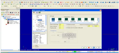
[image:8.612.179.432.238.351.2]

Figure2.3.3 shows the selection of tool path parameters in master cam

Figure 2.3.4 shows the pocketing type of tool path selection

Figure2.3.5 Show the optimization tool parameters

(9)

Technology (IJRASET)

Figure2.3.7 shows cutting simulations of object

Figure2.3.8 shows the fist type i.e zigzag tool path generation

(10)

Technology (IJRASET)

Figure2.3.10 shows the constant spiral tool path generation

Figure2.3.11 shows the tool path generation one-way

D. Tools Used

20 END MILL CARBIDE

20 END MILL HSS

10 END MILL HSS

10 END MILL CARBIDE

generated NC program for machining

%

O0000(R1)

(DATE=DD-MM-YY - 28-07-15 TIME=HH:MM - 17:17) (MCX FILE - T)

(NC FILE - C:\DOCUMENTS AND SETTINGS\KRISHNA\DESKTOP\R1.NC) (MATERIAL - ALUMINUM MM – 6061-T6)

( T219 | 10. FLAT ENDMILL | H219 ) N100 G21

N102 G0 G17 G40 G49 G80 G90 N104 T219 M6

N106 G0 G90 G54 X-31.75 Y3.75 S1909 M3 N108 G43 H219 Z25.

(11)

Technology (IJRASET)

N112 G1 Z-.5 F190.9 N114 M98 P1001 N116 G0 G90 Z24.5 N118 X-33. Y10. N120 Z2.

N122 G1 Z-.5 F190.9 N124 M98 P1002 N126 G0 G90 Z24.5 N128 X-31.75 Y3.75 N130 Z2.

N132 G1 Z-1. F190.9 N134 M98 P1001 N136 G0 G90 Z24. N138 X-33. Y10. N140 Z2.

N142 G1 Z-1. F190.9 N144 M98 P1002 N146 G0 G90 Z24. N148 X-31.75 Y3.75 N150 Z2.

N152 G1 Z-1.5 F190.9 N154 M98 P1001 N156 G0 G90 Z23.5 N158 X-33. Y10. N160 Z2.

N162 G1 Z-1.5 F190.9 N164 M98 P1002 N166 G0 G90 Z23.5 N168 X-31.75 Y3.75 N170 Z2.

(12)

Technology (IJRASET)

N210 Z2.

(13)

Technology (IJRASET)

N308 X-31.75 Y3.75 N310 Z2.

(14)

Technology (IJRASET)

N406 G0 G90 Z17.5 N408 X-31.75 Y3.75 N410 Z2.

(15)

Technology (IJRASET)

N504 M98 P1002 N506 G0 G90 Z25. N508 M5

N510 G91 G28 Z0. N512 G28 X0. Y0. N514 M30

O1001 N100 G91

N102 Y-7.5 F381.8 N104 Y-.858

N106 G2 X-1.716 R.858 N108 X.858 Y.858 R.858 N110 G1 X.858

N112 X64. N114 X.858

N116 G2 Y-1.716 R.858 N118 X-.858 Y.858 R.858 N120 G1 Y.858

N122 Y7.5 N124 Y.858

N126 G2 X1.716 R.858 N128 X-.858 Y-.858 R.858 N130 G1 X-.858

N132 X-64. N134 X-3.75 Y3.75 N136 Y-15. N138 Y-.858

N140 G2 X-1.716 R.858 N142 X.858 Y.858 R.858 N144 G1 X.858

N146 X71.5 N148 X.858

N150 G2 Y-1.716 R.858 N152 X-.858 Y.858 R.858 N154 G1 Y.858

N156 Y15. N158 Y.858

N160 G2 X1.716 R.858 N162 X-.858 Y-.858 R.858 N164 G1 X-.858

N166 X-71.5 N168 X-7.5 Y7.5 N170 Y-30. N172 Y-.858

(16)

Technology (IJRASET)

N182 X.858

N184 G2 Y-1.716 R.858 N186 X-.858 Y.858 R.858 N188 G1 Y.858

N190 Y30. N192 Y.858

N194 G2 X1.716 R.858 N196 X-.858 Y-.858 R.858 N198 G1 X-.858

N200 X-86.5 N202 X-7.5 Y7.5 N204 Y-45. N206 X101.5 N208 Y45. N210 X-101.5 N212 M99

O1002 N100 G91

N102 X-10. F381.8 N104 G3 X-10. Y-10. R10. N106 G1 Y-25.

N108 X106.5 N110 Y50. N112 X-106.5 N114 Y-25.

N116 G3 X10. Y-10. R10. N118 G1 X10.

N120 M99 %

E. Practical Work For The Present Project

Raw material;

1) Total components: 4 components-final sizes-120x40x25

(17)

Technology (IJRASET)

So raw material will be taken in to multiple with 10mm each side for making right angle. i.e. 150x50x35-4 ocks

[image:17.612.168.444.115.296.2]

2) The raw material should be maintained to right angle to each face.

Figure 2.5.2 shows the right angle of raw material cross section

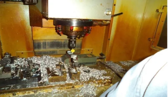
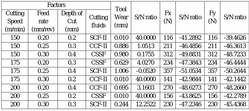
[image:17.612.169.446.337.490.2]

The machining process showed while machining the component with normal coolant with carbide end mill of 20 diameter to make size of 120x40x25.

[image:17.612.166.448.508.706.2]

(18)

Technology (IJRASET)

[image:18.612.168.448.100.265.2]

3) After the machining of final sizes the component is going to semi finishing because the wall thickness is very less.

Figure 5.3.5 shows the rough tool path with different tool paths for taguchi method S/N ratios.

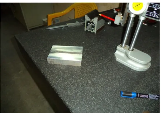
4) Before going to the final machining the specimen component checked for warp age and considered that the distortion before final machining is zero and after semi-finishing the value is zero on wall itself.

Figure 5.3.6 shows the finished component inspection on machine

III. TAGUCHI TESTING METHODOLOGY

A. Taguchi’s Technique

Taguchi’s comprehensive system of quality engineering is one of the greatest engineering achievements of the 20th century. His methods focus on the effective application of engineering strategies rather than advanced statistical techniques. It includes both upstream and shop-floor quality engineering. Upstream methods efficiently use small-scale experiments to reduce variability and remain cost-effective, and robust designs for large-scale production and market place. Shop-floor techniques provide cost-based, real time methods for monitoring and maintaining quality in production. The farther upstream a quality method is applied, the greater leverages it produces on the improvement, and the more it reduces the cost and time. Taguchi’s philosophy is founded on the following three very simple and fundamental concepts:

1) Quality should be designed into the product and not inspected into it.

2) Quality is best achieved by minimizing the deviations from the target. The product or process should be so designed that it is immune to uncontrollable environmental variables.

3) The cost of quality should be measured as a function of deviation from the standard and the losses should be measured system-wide.

[image:18.612.171.446.310.469.2]

(19)

Technology (IJRASET)

salvaging. No amount of inspection can put quality back into the product. Taguchi recommends a three-stage process: system design, parameter design and tolerance design. In the present work Taguchi’s parameter design approach is used to study the effect of parameters on the various responses of the mechanical strength.

B. Loss Function

The heart of Taguchi method is his definition of the nebulous and elusive term “quality” as the characteristic that avoids loss to the society from the time the product is shipped. Loss is measured in terms of monetary units and is related to quantifiable product characteristic.

Taguchi defines quality loss via his „loss function. He unites the financial loss with the functional specification through a quadratic relationship that comes from a Taylor series expansion. The quadratic function takes the form of a parabola. Taguchi defines the loss function as a quantity proportional to the deviation from the nominal quality characteristic. He has found the following quadratic form to be a useful workable function

L(y) =k(y-m)2 (3.1)

Where,

L = Loss in monetary units

m = value at which the characteristic should be set

y = actual value of the characteristic

k = constant depending on the magnitude of the characteristic and the monetary unit involved

The loss function represented in Eq. 3.1 is graphically shown in Figure 3.2. The characteristics of the loss function are

1) The farther the product’s characteristic varies from the target value, the greater is the loss. The loss must be zero when the quality characteristic of a product meets its target value.

2) The loss is a continuous function and not a sudden step as in the case of traditional approach (Figure 3.2). This consequence of the continuous loss function illustrates the point that merely making a product within the specification limits does not necessarily mean that product is of good quality.

a) Average loss-function for product population

In a mass production process, the average loss per unit is expressed as Figure 3.1 Taguchi Loss Function

(20)

Technology (IJRASET)

L(y) = {k(y1-m)2+k(y2-m)2+………..+k(yn-m)2} (3.2)

y1,y2…yn = Actual value of the characteristic for unit 1, 2,…n respectively

n = Number of units in a given sample

k = Constant depending on the magnitude of the characteristic and the

monetary unit involved

m = Target value at which the characteristic should be set

The Eq. 4.2 can be simplified as:

L(y) = k(MSDNB)

Where,

MSDNB = Mean squared deviation or the average of squares of all deviations from the

target or nominal value

NB = “Nominal is Best”

b) Other loss functions: The loss-function can also be applied to product characteristics other than the situation where the nominal value is the best value (m).

The loss-function for a “smaller is better” type of product characteristic (LB) is shown in Figure 4.2a. The loss function is identical to the „nominal-is-best type of situation when m=0, which is the best value for „smaller is better characteristic (no negative value). The loss function for a “larger-is-better” type of product characteristic (HB) is also shown in Figure 4.2b, where also m=0.

C. Signal To Noise Ratio

The loss-function discussed above is an effective figure of merit for making engineering design decisions. However, to establish an appropriate loss-function with its k value to use as a figure of merit is not always cost-effective and easy. Recognizing the dilemma, Taguchi created a transform function for the loss-function which is named as signal -to-noise (S/N) ratio

The S/N ratio, as stated earlier, is a concurrent statistic. A concurrent statistic is able to look at two characteristics of a distribution and roll these characteristics into a single number or figure of merit. The S/N ratio combines both the parameters (the mean level of the quality characteristic and variance around this mean) into a single metric

A high value of S/N implies that signal is much higher than the random effects of noise factors. Process operation consistent with highest S/N always yields optimum quality with minimum variation.

The S/N ratio consolidates several repetitions (at least two data points are required) into one value. The equation for calculating S/N ratios for „smaller is better (LB), „larger is better (HB) and „nominal is best (NB) types of characteristics are as follows

1) Larger the Better

()HB = -10 log(MSDHB)

Where,

MSDHB =

2) Smaller the Better

(21)

Technology (IJRASET)

Where,

MSDLB =)

3) Nominal the Best

()NB = -10 log(MSDNB)

Where,

MSDNB =

R = Number of repetitions

The mean squared deviation (MSD) is a statistical quantity that reflects the deviation from the target value. The expressions for MSD are different for different quality characteristics. For the „nominal is best characteristic, the standard definition of MSD is used. For the other two characteristics the definition is slightly modified. For „smaller is better, the unstated target value is zero. For „larger is better, the inverse of each large value becomes a small value and again, the unstated target value is zero. Thus for all three expressions, the smallest magnitude of MSD is being sought.

D. Relation Between S/N Ratio And Loss Function

Figure 4.2a shows a single sided quadratic loss function with minimum loss at the zero value of the desired characteristic. As the value of y increases, the loss grows. Since, loss is to be minimized the target in this situation for y is zero The basic loss function is:

L(y)=k(y-m)2

If m = 0

L(y)=k(y2 )

The loss may be generalized by using k=1 and the expected value of loss may be found by summing all the losses for a population and dividing by the number of samples R taken from this population. This in turn gives the following expression

EL = Expected loss =(∑y2∕R)

The above expression is a figure of demerit. The negative of this demerit expression produces a positive quality function. This is the thought process that goes into the creation of S/N ratio from the basic quadratic loss function. Taguchi adds the final touch to this transformed loss-function by taking the log (base 10) of the negative expected loss and then he multiplies by 10 to put the metric into the decibel terminology 52 The final expression for “smaller-is-better” S/N ratio takes the form of Equation 4.2. The same thought pattern follows in creation of other S/N ratios.

E. Experimental Design Strategy

Taguchi recommends orthogonal array (OA) for laying out of experiments. These OA‟s are generalized Graeco-Latin squares. To design an experiment is to select the most suitable OA and to assign the parameters and interactions of interest to the appropriate columns. The use of linear graphs and triangular tables suggested by Taguchi makes the assignment of parameters simple. The array forces all experimenters to design almost identical experiments. In the Taguchi method the results of the experiments are analyzed to achieve one or more of the following objectives

1) To establish the best or the optimum condition for a product or process

2) To estimate the contribution of individual parameters and interactions

3) To estimate the response under the optimum condition

(22)

Technology (IJRASET)

confidence. Study of ANOVA table for a given analysis helps to determine which of the parameters need control. Taguchi suggests two different routes to carry out the complete analysis. First, the standard approach, where the results of a single run or the average of repetitive runs are processed through main effect and ANOVA analysis (Raw data analysis). The second approach which Taguchi strongly recommends for multiple runs is to use signal- to- noise ratio (S/N) for the same steps in the analysis. The S/N ratio is a concurrent quality metric linked to the loss function. By maximizing the S/N ratio, the loss associated can be minimized. The S/N ratio determines the most robust set of operating conditions from variation within the results. The S/N ratio is treated as a response (transform of raw data) of the experiment. Taguchi recommends the use of outer OA to force the noise variation into the experiment i.e. the noise is intentionally introduced into experiment. However, processes are often times subject to many noise factors that in combination, strongly influence the variation of the response. For extremely “noisy” systems, it is not generally necessary to identify specific noise factors and to deliberately control them during experimentation. It is sufficient to generate repetitions at each experimental condition of the controllable parameters and analyze them using an appropriate S/N ratio.

In the present investigation, the raw data analysis and S/N data analysis have been performed. The effects of the selected process parameters on the selected quality characteristics have been investigated through the plots of the main effects based on raw data. The optimum condition for each of the quality characteristics has been established through S/N data analysis aided by the raw data analysis. No outer array has been used and instead, experiments have been repeated three times at each experimental condition.

F. Steps In Experimental Design And Analysis

The important steps are discussed in the subsequent article.

1) Selection of orthogonal array (OA): In selecting an appropriate OA, the pre-requisites are

a) Selection of process parameters and/or interactions to be evaluated

b) Selection of number of levels for the selected parameters

The determination of parameters to be investigated hinges upon the product or process performance characteristics or responses of interest. Several methods are suggested by Taguchi for determining which parameters to include in an experiment. These are

i. Brainstorming

ii. Flow charting

iii. Cause-Effect diagrams

The total Degrees of Freedom (DOF) of an experiment is a direct function of total number of trials. If the number of levels of a parameter increases, the DOF of the parameter also increases because the DOF of a parameter is the number of levels minus one. Thus, increasing the number of levels for a parameter increases the total degrees of freedom in the experiment which in turn increases the total number of trials. Thus, two levels for each parameter are recommended to minimize the size of the experiment If curved or higher order polynomial relationship between the parameters under study and the response is expected, at least three levels for each parameter should be considered (Barker, 1990). The standard two level and three level arrays are

i. Two level arrays: L4, L8, L12, L16, L32

ii. Three level arrays : L9, L18, L27

The number as subscript in the array designation indicates the number of trials in that array. The total degrees of freedom (DOF) available in an OA are equal to the number of trials minus one

= N-1 Where,

=Total degrees of freedom of an OA LN = OA designation

N = Number of trials

When a particular OA is selected for an experiment, the following inequality must be Satisfied ≥ Total degree of freedom required for parameters and interactions

Depending on the number of levels of the parameters and total DOF required for the experiment, a suitable OA is selected. The OA”s has several columns available for assignment of parameters and some columns subsequently can estimate the effect of interactions of these parameters. Taguchi has provided two tools to aid in the assignment of parameters and interactions to arrays

i. Linear graphs

(23)

Technology (IJRASET)

Each OA has a particular set of linear graphs and a triangular table associated with it. The linear graphs indicate various columns to which parameters may be assigned and the columns subsequently evaluate the interaction of these parameters. The triangular tables contain all the possible interactions between parameters (columns). Using the linear graphs and /or the triangular table of the selected OA, the parameters and interactions are assigned to the columns of the OA.

Selection of outer array

Taguchi separates factors (parameters) into two main groups: controllable factors and uncontrollable factors (noise factors). Controllable factors are factors that can easily be controlled. Noise factors, on the other hand, are nuisance variables that are difficult, impossible, or expensive to control. The noise factors are responsible for the performance variation of a process. Taguchi recommends the use of outer array for the noise factors and inner arrays for controllable factors. If an outer array is used, the noise variation is forced into the experiment. However, experiments against the trial conditions of the inner array (the OA used for the controllable factors) may be repeated and in this case the noise variation is unforced into the experiment The outer array, if used, will have same assignment considerations. However, the outer array should not be complex as the inner array because the outer array is noise only which is controlled only in the experiment. An example of inner and outer array combination.

G. Experimentation And Data Collection

The experiment is performed against each of the trial conditions of the inner array. Each experiment at a trial condition is repeated simply (if outer array is not used) or according to the outer array (if used). Randomization should be carried to reduce bias in the experiment.

The data (raw data) are recorded against each trial condition and S/N ratios of the repeated data points are calculated and recorded against each trial condition

H. Data Analysis

A number of methods have been suggested by Taguchi for analyzing the data: observation method, ranking method, column effect method, ANOVA, S/N ANOVA, plot of average response curves, interaction graphs etc. However, in the present investigation the following methods have been used:

1) Plot of average response curves

2) ANOVA for raw data

3) ANOVA for S/N data

4) S/N response graphs

[image:23.612.193.421.590.703.2]

The plot of average responses at each level of a parameter indicates the trend. It is a pictorial representation of the effect of parameter on the response. The change in the response characteristic with the change in levels of a parameter can easily be visualized from these curves. Typically, ANOVA for OA”s are conducted in the same manner as other structured experiments. The S/N ratio is treated as a response of the experiment, which is a measure of the variation within a trial when noise factors are present. A standard ANOVA can be conducted on S/N ratio which will identify the significant parameters (mean and variation). Interaction graphs are used to select the best combination of interactive parameters The experimental results are analyzed using Taguchi method and the significant parameters affecting material have to be identified. The results of the Taguchi analysis are presented in results and discussion chapter.

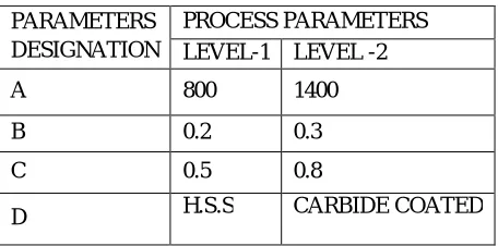
Table 3.1Process parameters with their values at 2 levels.

PARAMETERS DESIGNATION

PROCESS PARAMETERS LEVEL-1 LEVEL -2

A 800 1400

B 0.2 0.3

C 0.5 0.8

(24)

Technology (IJRASET)

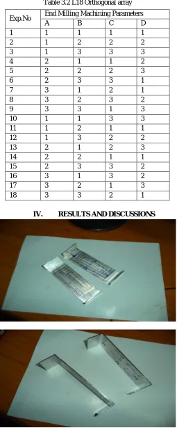
Table 3.2 L18 Orthogonal array

IV. RESULTS AND DISCUSSIONS

Fig.4.1 & 4.2 shows the quality checking values of specimen Exp.No End Milling Machining Parameters

A B C D

1 1 1 1 1

2 1 2 2 2

3 1 3 3 3

4 2 1 1 2

5 2 2 2 3

6 2 3 3 1

7 3 1 2 1

8 3 2 3 2

9 3 3 1 3

10 1 1 3 3

11 1 2 1 1

12 1 3 2 2

13 2 1 2 3

14 2 2 1 1

15 2 3 3 2

16 3 1 3 2

17 3 2 1 3

[image:24.612.180.435.79.694.2]

(25)

Technology (IJRASET)

A. Quality Check Before Releasing From Fixture

The value taken at the centre is 0.000 and the distortion checked at 4 ends as left middle, right middle, top end, top-y, bottom y. left wall top, right wall top, overall maximum distortion. The final values are shown in table

Table 4.1 is showing values before releasing from fixture

Specimen-1 0.010 0.010 0.010 0.010 0.040 0.020 0.020 0.010 0.025

Specimen-2 0.010 0.020 0.020 0.010 0.050 0.020 0.010 0.010 0.020 Specimen-3 0.030 0.020 0.040 0.030 0.050 0.040 0.030 0.040 0.040 Specimen-4 0.050 0.055 0.050 0.040 0.040 0.050 0.040 0.050 0.050

B. Quality Check After Releasing From Fixture

The final results are shown in table 4.2 Table 4.2 is showing values after releasing from fixture

Specimen-1 0.020 0.020 0.050 0.050 0.075 0.070 0.055 0.050 0.060 Specimen-2 0.030 0.030 0.030 0.040 0.060 0.060 0.050 0.050 0.050 Specimen-3 0.080 0.060 0.010 0.080 0.075 0.075 0.060 0.060 0.080 Specimen-4 0.050 0.055 0.100 0.100 0.075 0.050 0.060 0.060 0.085

C. Distortion Graphs

4.3 showing Distortion Graphs

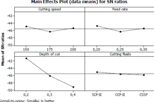
[image:25.612.96.504.546.729.2]

D. VALUES OF S/N RATIOS FOR TOOL WEAR, Fx AND Fy’s

Table 4..3.1 summary of S/N ratios for tool wear, Fx and Fy’s Factors

Tool Wear (mm)

S/N ratio Fx

(N) S/N ratio Fy

(N) S/N ratio Cutting Speed (m/min) Feed rate (mm/rev) Depth of Cut (mm) Cutting fluids

150 0.20 0.2 SCF-II 0.010 40.0000 116 -41.2892 116 -39.4626 150 0.25 0.3 CCF-II 0.886 1.0513 211 -46.4856 211 -46.3613 150 0.30 0.4 CSSF 0.980 0.1755 312 -49.8831 312 -48.7233 175 0.20 0.3 CSSF 0.629 4.0270 234 -47.3843 234 -46.4444 175 0.25 0.4 SCF-II 1.006 -0.0520 357 -51.0534 357 -50.2644 175 0.30 0.2 CCF-II 0.010 40.0000 141 -42.9844 141 -42.1442 200 0.20 0.4 CCF-II 0.695 3.1603 270 -48.6273 270 -48.2660 200 0.25 0.2 CSSF 0.010 40.0000 156 -43.8625 156 -42.2789

0 0.05 0.1 0.15 0.2

15 30 45 60 75 90 110130150 case4

case3

case2

case1 Distortion

(26)

[image:26.612.181.429.83.247.2]

Technology (IJRASET)

Figure 4.4Specimen 1S/N ratios graph with speed and feed

E. Analysis Of Variance (ANOVA)

ANOVA was used to determine the significant parameters influencing the tool wear and force components in the milling of AISI 304. Tables5.4 showed the summary of S/N values and ANOVA results for tool wear, Fx and Fy, respectively.

Tables4.4 Summary of S/N values and ANOVA results for Fx

Factor

Degree of Freedom (DF)

Average S/N Values

Sum of squares Mean square Percentage of contribution (%) Level 1 Level

2 Level3

Cutting speed 2

-45.89

-47.14 -46.57 1634.9 870.3 3.20 Feed

rate 2

-45.79

-47.13 -46.70 1829.6 922.3 3.59 Depth

of cut 2

-42.71

-47.03 -49.85 46112.8 23056.4 90.39 Cutting

fluids 2

-46.53

-46.03 -47.04 1440.2 720.1 2.82

Error 0 0

Total 8 51017.5 100

Tables4.5 Summary of S/N values and ANOVA results for Fy

Tables4.6 Summary of S/N values and ANOVA results for Tool Wear Factor Degree

of Freedom (DF)

Average S/N Values Sum of squares Mean square Percentage of contribution (%) Level 1 Level 2 Level3 Cutting speed

2

-44.85 -46.28

-45.28 1740.7 870.3 3.76

Feed rate

2

-44.76 -46.30

-45.28 1844.7 922.3 3.98

Depth of cut

2

-41.20 -46.05

-49.05 42672.7 21336.3 92.14

Cutting fluids

2

-45.73 -45.81

(27)

Technology (IJRASET)

Factor Degree of Freedom (DF)

Average S/N Values Sum of squares Mean square Percentage of contribution (%) Level 1 Level 2 Level3 Cutting speed

2 13.742 14.658 18.471 0.15523 0.07762 10.52

Feed rate

2 15.729 13.666 17.476 0.08654 0.04327 5.86

Depth of cut

2 40.000 5.777 1.095 1.20758 0.60374 81.82

Cutting fluids

2 17.4 14.737 14.734 0.02658 0.01329 1.80

Error 0 0

Total 8 46314.0 100

In this study, analysis was a level of significance as 5% and level of confidence as 95%.

V. CONCLUSIONS

A. Studied the differential variation in m/c by using carbide and HSS tools. Carbide tool on more effective than HSS because of vibrating nature (modules of elasticity is more for HSS)

B. Two step m/c process reliable for open loops. i.e, shaped profiles. Semi m/c will reduce internal stresses due to the read on distortion will be decreased.

C. Production coolant is also important to reduce that generation write machining comparing to all other coolants. Coolant is more reliable for can bide and coolant is mixed with water in reliable for HSS.

D. Distortion is reduced when the work price machining with carbide h using coolant as oil. When compare to other procedures.

E. Carbide tools and coolant oil in a little expensive than other procedures but when compare to quality analysis the above two is reliable. So, it can increases production rate without component rejection.

VI. FUTURE SCOPE

A. Can calculate differentiation in direction and semi finish with finish.

B. Can use one tool for all specimens for – above conclusion.

C. Can check the m/c process with low cost tool like h. s s. With different tool path.

D. Can change the material with different composition, different needs by following procedures. REFERENCES

[1] Nithyanandhan T. et al “Optimization of Cutting Forces, Tool Wear and Surface Finish in Machining of AISI 304 Stainless Steel Material Using Taguchi’s Method”, International Journal of Innovative Science, Engineering & Technology, Vol. 1 Issue 4, June 2014, page 488-493.

[2] Samrudhi Rao et al “An Overview of Taguchi Method: Evolution, Concept and Interdisciplinary Applications”, International Journal of Scientific & Engineering Research, Volume 4, Issue 10, October-2013, page 621-626.

[3] Quazi T Z et al “a case study of Taguchi method in the optimization of turning parameters”, International Journal of Emerging Technology and Advanced Engineering Volume 3, Issue 2, February 2013, page 616-626.

[4] Atul Kulkarni et al “Design optimization of cutting parameters for turning of AISI 304 austenic stainless steel using Taguchi method”, Indian Journal of engineering & material sciences, vol. 20, August 2013, page 252-258 .

[5] Vikas B. Magdum et al “Evaluation and Optimization of Machining Parameter for turning of EN 8 steel”, International Journal of Engineering Trends and Technology (IJETT) - Volume4 Issue5- May 2013, page 1564-1568.

[6] Krishankant et al “Application of Taguchi Method for Optimizing Turning Process by the effects of Machining Parameters”, International Journal of

Error 0 0

(28)

Technology (IJRASET)

01, No. 01, May 2011, page 44-46.

[8] D. Philip Selvaraj , P. Chandramohan “Optimization Of Surface Roughness of Aisi 304 Austenitic Stainless Steel In Dry Turning Operation Using Taguchi Design Method” Journal of Engineering Science and Technology Vol. 5, No. 3 (2010) 293 – 301.

[9] Elso Kuljanic et al “Machinability of difficult machining materials”, 14th International Research/Expert Conference “Trends in the Development of Machinery and Associated Technology” TMT 2010, Mediterranean Cruise, 11-18 September 2010, page I-1 to I-14

[10] E. Kuram, “Investigation of vegetable-based cutting fluids performance in drilling,” M.Sc. Thesis, Gebze Institute of Technology, Gebze, Turkey, 2009. [11] L. De Chiffre, and W. Belluco, “Investigations of cutting fluid performance using different machining operations,” Lubri. Eng., vol. 58, pp. 22-29, 2002. [12] M. A. Xavior, and M. Adithan, “Determining the influence of cutting fluids on tool wear and surface roughness during turning of AISI 304 austenitic stainless

(29)