Guidelines for benchmarking of optimization based approaches for fitting mathematical models

R E V I E W

Open Access

Guidelines for benchmarking of

optimization-based approaches for fitting

mathematical models

Clemens Kreutz

Abstract

Insufficient performance of optimization-based approaches for the fitting of mathematical models is still a major bottleneck in systems biology. In this article, the reasons and methodological challenges are summarized as well as their impact in benchmark studies. Important aspects for achieving an increased level of evidence for benchmark results are discussed. Based on general guidelines for benchmarking in computational biology, a collection of tailored guidelines is presented for performing informative and unbiased benchmarking of optimization-based fitting approaches. Comprehensive benchmark studies based on these recommendations are urgently required for the establishment of a robust and reliable methodology for the systems biology community.

Keywords: Benchmarking, Differential equation models, Optimization, Parameter estimation, Systems biology

Introduction

A broad range of mathematical models is applied in sys-tems biology. Depending on the questions of interest and on the amount of available data, the type of models and the level of detail vary. Most frequently,ordinary differential equation models (ODEs)are applied because they enable a non-discretized description of the dynamics of a system and allow for quantitative evaluation of experimental data including statistical interpretations in terms of confidence and significance. In theBioModels Database[1], currently, 83% of all models which are uniquely assigned to a mod-eling approach are ODE models. In this article, I focus on the optimization-based fitting of these models although many aspects are general and also apply to other modeling types and approaches.

Typical parameters in systems biology such as the abun-dances of compounds or the strengths and velocities of biochemical interactions are typically context-dependent, i.e., they vary between species, tissues, and cell types. Hence, they are represented as unknown parameters in mathematical models. Application-specific calibration of

Correspondence:[email protected]

1_{Faculty of Medicine and Medical Center, Institute of Medical Biometry and}

Statistics, University of Freiburg, Stefan-Meier-Str. 26, 79104 Freiburg, Germany 2_{CIBSS–Centre for Integrative Biological Signalling Studies, University of}

Freiburg, Freiburg, Germany

the models is therefore required which corresponds to the estimation of these unknown parameters based on experimental data.

In most cases, parameter estimation is performed by the optimization of a suitableobjective functionsuch as mini-mization of the sum of squared residuals forleast squares

estimation or maximization of the likelihood for max-imum likelihood estimation [2]. Both approaches coin-cide with normally distributed measurement errors. Such optimization-based fitting of a model requires the selec-tion of a generic numerical optimizaselec-tion approach as a core algorithm. In addition, the optimization problem needs to be defined in terms of initialization, search space, termination criteria, andhyperparametersthat set up and configure the numerical algorithms. Although parameter estimation is a central task of modeling, the lack of reliable computational approaches for fitting is still a bottleneck in systems biology. The absence of high-performing soft-ware implementations seems to be a major reason why ODE-based modeling is not yet a routinely applied com-putational approach for analyzing experimental data.

The importance of proper designs for benchmark stud-ies in computational biology has been discussed in several publications [3–5]. General guidelines have been provided recently for computational analysis of omics data [6], mul-tiple alignment of protein sequences [7], and supervised

which is also termed calibration or model calibration in the literature.

Why is reliable fitting challenging?

A major characteristic of the mathematical models applied in systems biology is the intention to mirror the biological process of interest because this facilitates enhanced possibilities of interpretations and understand-ing. To this end, molecular compounds such as proteins and spatial compartments such as cells are defined as model components. Moreover, biochemical interactions between the considered compounds are translated as rate equations into the model. In contrast to phenomenologi-calmodels which describe the empirical relationships in an abstract and simplified manner, the complexity of these so-calledmechanisticmodels is dictated by the complexity of the investigated biological process.

Estimating the parameters of typical models in sys-tems biology requires data that covers a broad set of experimental conditions such as multiple time points, genetic perturbations, and/or treatments. Since the eval-uation of distinct experimental conditions is elaborate, the amount of available experimental data for param-eter estimation is always limited. In such kind of set-tings, multiple parameter combinations can give rise to the same model response for experimentally investigated conditions. A measured steady-state concentration, for instance, might merely provide information about the ratio kprod/kdeg of production and degradation rates.

Because different combinations of the individual param-eters kprod and kdeg result in the same steady state, all

combinations with the same ratio fit the data equally well. Such sub-spaces where the objective function is entirely flat has been termed non-identifiability. Because non-identifiability is common features of models in systems biology, the equations which have to be solved during optimization are ill-conditioned or even have non-unique solutions which decreases the performance of numerical algorithms.

The following typical attributes of mechanistic models in systems biology raise methodological challenges for the model fitting:

(a) The models are large in terms of the number of parameters and dynamic variables. Thus,

the numerical integration of the ODEs which is computationally demanding and only feasible with limited numerical accuracy.

(d) Because explicit solutionsx(t)for the ODEsx˙=f(x)

cannot be derived by analytical calculations, all mathematical calculations requiringx(t)in an explicit form are infeasible.

(e) Derivatives of the objective function have limited numerical accuracy and cannot be calculated naively. (f) Parameter values vary over several orders of

magnitudes, and usually, only a limited amount of prior knowledge is available. Therefore, it is difficult to specify priors, initial guesses, and/or bounds. (g) Optimization has to cope with constraints like upper

and lower bounds and with non-identifiability, i.e., with ill-conditioning and entirely flat sub-spaces.

In addition, discontinuities of external inputs (so-called

events) [13] might occur which has to be handled properly. Sometimes, steady-state constraints for the initial values have to be implemented numerically which is another source of performance loss [14].

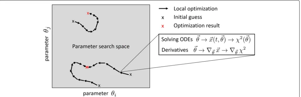
Fig. 1Tasks to be accomplished for fitting ODE models. The fitting of ODE models requires several generic tasks. The optimization problem has to be defined in terms of bounds of the search space and geometry (e.g., linear vs. log scale). Moreover, the selected generic optimization algorithm applied as the core of optimization-based fitting has to be initialized. There are many ways of combining global and local search strategies. A prominent global search strategy is random drawing of multiple initial guesses and performing local optimization for each starting point. In each optimization step of a local optimization run, the ODEs have to be solved for the evaluation of the objective function_χ2_{(θ). Incremental} improvement strategies are applied for suggesting a new parameter vector for the next iteration step in the core optimization routine which is usually performed based on derivatives or approximations thereof

An early publication in systems biology found superior performance of the so-called multiple shooting [17] for local optimization. The idea behind multiple shooting is to reduce the non-linear dependency on the parameters by partitioning time courses into multiple short inter-vals. Yet, this method is difficult or even impossible to apply for partly observed systems with complex observa-tion funcobserva-tions. It requires a custom implementaobserva-tion of an ODE integration method, and its combination with global search strategies has not been considered. Moreover, there are no implementations publicly available. Consequently, this methodology disappeared from the systems biology field during recent years.

Repeating deterministic optimization runs for multi-ple initial guesses, i.e., so-called multi-start optimiza-tion, showed superior performance in the Dialogue for Reverse Engineering Assessments and Methods (DREAM)

benchmark challenges about parameter estimation [18] and network reconstruction [19]. Here, a trust region

and gradient-based deterministic non-linear least squares optimization approach [20] has been utilized as a local optimization strategy, and a global search was performed by utilizing multiple runs with random initial guesses. Trust regions are iteratively updated confidence areas indicating sufficient quality of the local approximation of the objective function which yields successful opti-mization steps. This approach is implemented in the

Data2Dynamicsmodeling framework [21] and proved to be superior to other approaches in several studies [22–24]. It has been shown that deterministic gradient-based optimization is superior to a batch of stochastic algorithms and hybrid approaches which combine deterministic and stochastic search strategies [22]. In

contrast, other studies found superior performance of stochastic optimization methods [25–28]. It was con-firmed that multi-start gradient-based local optimization is often a successful strategy [29], but on average, a better performance could be achieved with a hybrid meta-heuristic [25] combining deterministic gradient-based optimization with a global scatter search metaheuristic.

Finite differences(F(θ+h)−F(θ))/hwith step sizehare the most naive way of calculating a derivative of an objec-tive function F(θ) with respect to parameter θ. While it has been shown that derivative calculation based on finite differences is inappropriate for ODE models [22,30], this outcome has been partly questioned [31], at least if optimization is performed on a normalized data scale. In addition, for large models, the so-calledadjoint sensitivi-tieswere reported to be computationally most efficient for derivative calculations [30].

It has been repeatedly stated that parameters are prefer-ably optimized on the log scale [5,29,32]. Nevertheless, optimization of model parameters is still frequently per-formed at the linear scale in applications and even in benchmark studies [31].

atic errors which is usually not considered for simulated data sets. Simulating data for assessing model calibra-tion approaches requires much more specificacalibra-tions than in most other fields of computational biology. The rea-son for this is that realistic combinations of sampling times, observables, observation functions, error models, and experimental conditions have to be defined because this has a great impact on the amount of information pro-vided by the data. Moreover, in order to successfully reject incomplete model structures, it is necessary that the fit-ting of experimental data works for such wrong models as well. Since simulated data is typically generated with the same model structure used for fitting, there is usu-ally no mismatch between the model and the data. Thus, optimization is only evaluated for settings where a correct model structure is available. In order to not rely on such critical assumptions, it is highly preferable to assess fitting approaches based on real experimental data.

The common advantage of simulated data is the inher-ent knowledge about the underlying truth because this usually allows for appraisal in terms of true/false pos-itives or in terms of bias and variance. In contrast to most other benchmarking fields, this aspect is hardly relevant for benchmarking of optimization approaches because, on the one hand, each simulated data realiza-tion has a different, unknown optimum. Thus, the global solution is unknown even for simulated data. On the other hand, assessment by distance of estimated and true parameter values is not meaningful because of non-identifiability. Moreover, the outcomes of several opti-mization approaches can be assessed by evaluating the objective function which is feasible without any restriction for experimental data.

In real applications, there is only limited information available for initialization and for tuning of hyperpa-rameters, for instance, integration tolerances or thresh-olds defining termination criteria of iterative optimiza-tion. Therefore, default configurations have to be uti-lized or hyperparameters have to be defined by consis-tency checks. In benchmark studies, one has to strictly avoid tuning of such configurations based on the perfor-mance criteria in order to prevent unrealistic perforperfor-mance assessment. Instead, it should be prespecified before the evaluation of the methods of how hyperparameters will be chosen based on the information that is also available in

In our setting, the performance comparison of generic optimization approaches as the core of the fitting pro-cess is usually of primary interest. These approaches are typically available as different generic algorithms. How-ever, there are a lot of decisions which have to be made for applying those generic algorithms in the context of model calibration and thus appear as covariates: First, a set of benchmark problems has to be selected. More-over, a strategy for combining global and local search has to be specified, and an ODE integration method has to be selected. In addition, parameter bounds and parame-ter scales (linear vs. logarithmic) have to be defined and ODE integration algorithms and tolerances have to be specified as well as stopping the criteria for iterative opti-mization. Each of these decisions should be considered as a covariate.

The fact that these covariates affect the performance of individual core routines for optimization poses a severe problem. Wrong conclusions can be drawn since it is difficult to entirely uncover the origin of observed per-formance differences. In the example depicted in Fig.2, approach A requires properly tuned tolerances control-ling the accuracy of ODE integration. If properly chosen, this approach is superior. In contrast, approach B is less sensitive to these tolerances and outperforms A for most choices although the approach can never reach the max-imal performance possible for approach A. This example illustrates that observing a performance benefit of one approach for a specific tolerance merely provides a frag-mentary and possibly misleading picture.

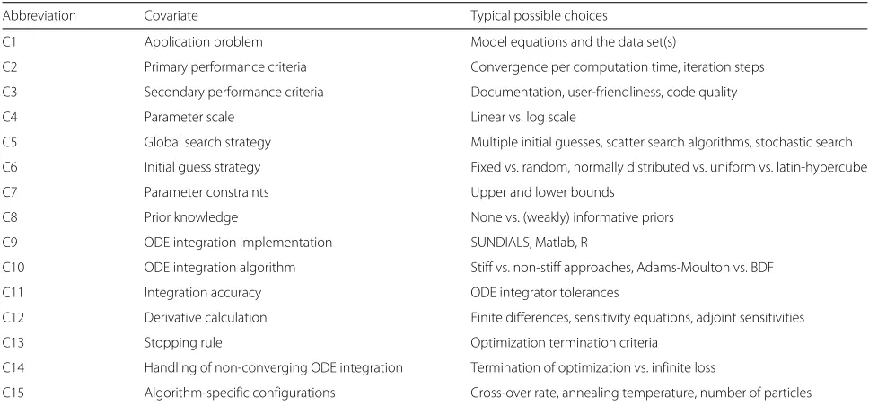
Analyzing multiple effects by a multi-variate statistical terminology is not yet common for benchmark stud-ies, but well-established, e.g., for clinical studies where patient-specific covariables such as gender, age, and smok-ing occur as covariates. Table 1 summarizes 15 typical covariates for optimization benchmark studies and illus-trates that many decisions have to be made for the imple-mentation of an optimization-based parameter estimation approach.

Fig. 2Impact of hyperparameters. Multiple configurations can have an impact on performance. In this illustration example, two optimization approaches have different sensitivities with respect to the choice of tolerances controlling the numerical error of ODE integration. Moreover, both approaches have different optimal choices for this hyperparameter. For most integration tolerances, approach B is superior. However, approach A displays the overall best performance for optimally chosen tolerances. This illustration example highlights the importance of the evaluation of hyperparameters for drawing valid conclusions

the full configuration space is not feasible for all relevant covariates. Nevertheless, the robustness of the conclu-sions with respect to the covariates has to be addressed, and limitations of the scope of the conducted studies should be kept in mind. A pragmatic way to achieve this is by verifying that changes of the individual covariates do not alter the outcome dramatically. Moreover, classical study design principles such as balancing and/or random-ization can be applied in order to minimize the impact of covariates [5]. As an example, one could randomly select many reasonable choices of all the covariates sum-marized in Table 1. To prevent bias due to imbalanced random drawings, one could draw the covariates jointly for all studied optimization algorithms to ensure that all

optimization algorithms are evaluated for the same set of covariates.

P3: Performing only case studies

The performance of optimization approaches depends on the application problem, i.e., on the models and the data sets which are used for benchmarking. A chosen bench-mark model determines the intricacy of the optimization task in terms of dimension (number of parameters), non-linearity, ill-conditioning, local optima, amount of infor-mation provided by the data, etc. and thereby affect the performance. Thus, the choice of application problems can be interpreted as an additional covariate that exhibits a strong effect on optimization performance.

Table 1Covariates

Abbreviation Covariate Typical possible choices

C1 Application problem Model equations and the data set(s)

C2 Primary performance criteria Convergence per computation time, iteration steps

C3 Secondary performance criteria Documentation, user-friendliness, code quality

C4 Parameter scale Linear vs. log scale

C5 Global search strategy Multiple initial guesses, scatter search algorithms, stochastic search

C6 Initial guess strategy Fixed vs. random, normally distributed vs. uniform vs. latin-hypercube

C7 Parameter constraints Upper and lower bounds

C8 Prior knowledge None vs. (weakly) informative priors

C9 ODE integration implementation SUNDIALS, Matlab, R

C10 ODE integration algorithm Stiff vs. non-stiff approaches, Adams-Moulton vs. BDF

C11 Integration accuracy ODE integrator tolerances

C12 Derivative calculation Finite differences, sensitivity equations, adjoint sensitivities

C13 Stopping rule Optimization termination criteria

C14 Handling of non-converging ODE integration Termination of optimization vs. infinite loss

C15 Algorithm-specific configurations Cross-over rate, annealing temperature, number of particles

conclusions.

P4: Non-convergence and local optima are hardly distinguishable

Sub-optimal convergence behavior is difficult to be dis-criminated from local optima since in both cases, the opti-mization terminates at distinct points in the parameter space, usually with different objective function values. In high-dimensional spaces, it is difficult to evaluate whether a point in the parameter space is a local optimum, especially if the objective function and its derivatives can only be evaluated with limited numeri-cal accuracy. Existing approaches which could be applied like the profile likelihood [33], reconstruction of flat manifolds [34], identifiability analysis [35], or methods

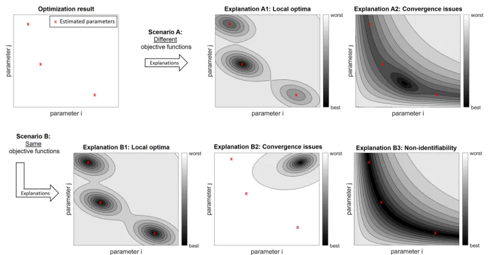
come of three optimization runs. “Scenario A” indicates that both convergence problems and local optima might generate the same observations. Even if identical values for the objective function are obtained (scenario B), the interpretation is ambiguous because there are no reli-able approaches to distinguish convergence issues from local optima. Moreover, the third possible explanation in this scenario is associated with non-identifiabilities, i.e., optimal sub-spaces. If non-identifiabilities exist, even high-performing optimization approaches converge to distinct points in the parameter space. For bench-mark analyses, this means that it is not reasonable to measure the similarity of the outcomes of multi-ple optimization runs by distances in the parameter space.

Fig. 3Ambiguous interpretation of optimization outcomes. For non-trivial optimization problems, the results of independent optimization runs are typically not the same. The upper left panel indicates an outcome for three optimization runs, e.g., generated with different starting points. If the objective function values after optimization are different (scenario A), such an outcome could be explained by local optima (explanation A1) or by convergence problems of the optimization algorithm (explanation A2). If the same values are obtained for objective function, there might be several local optima with the same value of the objective function (explanation B1), there might be a convergence problem (B2), or

Guidelines for benchmark studies

I recommend that the guidelines presented below are dis-cussed in future publications in a point-by-point manner in order to provide a summary for the readers about the design of a benchmark study and the resulting evidence in an easily accessible and clearly structured manner. Mul-tiple guidelines might be required to prevent a pitfall. Conversely, an individual guideline might help to prevent several pitfalls.

General guidelines for benchmark studies in the whole computational biology field have been recently presented [12]. Here, I concretize what those general sugges-tions mean for benchmarking of parameter optimization approaches and discuss their relevance, feasibility, and dif-ferences in our context. The terminology and order are kept as similar as possible to [12].

G1: Clear definition of aim and scope

Benchmark studies which are performed to illustrate the benefits of a newly presented approach are easily biased because they are performed to confirm merits. Often, application problems are utilized where existing methods have limited performance. Consequently, it should be pre-cisely stated whether benchmark analyses are performed for introducing a new approach, or whether the goal is performing a neutral and comprehensive study based on previously published computational approaches and test cases [5,12].

Since the performance of optimization routines is context-specific, i.e., depends on the chosen benchmark problem, it is essential to define the scope of a study and select representative test cases according to this def-inition [5]. For mathematical modeling in the systems biology field, one could define the scope by the bio-logical background. Models of signaling pathways, for instance, usually describe the dynamics of activation after stimulation and show transient dynamic responses. In contrast, metabolic models usually constitute steady-state descriptions. Gene regulatory networks, on the other hand, typically have distinct rate laws because activatory and inhibitory effects are described by products of Hill equations, instead ofmass action kinetics. Other options for defining scopes could be based on model attributes like the amount of data, number of parameters, existence of events, or steady-state constraints, or based on dynamic characteristics such as the occurrence of oscillations.

G2: Inclusion of (all) relevant methods

In contrast to other fields of computational biology, it is currently infeasible to include all relevant optimization methods in a benchmark study because published opti-mization methods are only available in distinct software or programming environments. In addition, optimization-based fitting of ODE models requires the combination of

several numerical tasks which do not perfectly coincide in different programming languages or software package. As an example, the trust region-based non-linear least square optimization approaches implemented in Matlab and R are not identically programmed and produce different outcomes with distinct performances [36].

Moreover, there is not yet an established standard for defining an optimization problem comprehensively including all model equations, data, measurement errors, priors, constraints, algorithms, and hyperparameters. Thus, it is very elaborate and partly infeasible to include approaches which are previously applied in other bench-mark studies. This limitation demands for standardized data and documentation formats likeCOMBINEarchives [37]. Nevertheless, including as many approaches as pos-sible is an important and indispenpos-sible aim. For rea-sonable interpretation of observed performances, it is absolutely essential to implement at least one state-of-the-art approach and to verify that the implementation or the observed performance is coinciding with previous benchmark studies.

G3: Selection of realistic and representative test cases

Because the performance of optimization approaches strongly varies between the application models, a rather large number of models is required to obtain a repre-sentative and comprehensive set of test cases. However, the number of available benchmark problems is very lim-ited so far. Six benchmark models have been published in [38]; however, four of them only contain simulated data. Recently, a set of 20 benchmark problems with exper-imental data sets has been published [32], but it still remains difficult to perform larger benchmark studies. Because of the small number of available test cases, it is currently only hardly feasible to define a narrow scope of such a study while still including enough test problems.

Simulation of data is valuable for understanding and validation of an observed performance loss in bench-mark studies. However, as argued above as pitfall P1, simulated data has only limited value for benchmarking of optimization-based fitting approaches. Hence, bench-mark studies based on experimental data are more repre-sentative and thus are strongly recommended.

G4: Appropriate hyperparameters and software versions

age as well as their impact have not been investigated yet. Nevertheless, in order to guarantee full reproducibil-ity, it is essential to comprehensively describe the applied approach including software versions. Software tools for enhancing the reproducibility of computational analyses have been summarized previously [12].

G5: Evaluation in terms of key quantitative metrics

Optimization is in almost all circumstances assessed by means of convergence, i.e., in terms of probabilities or frequencies of finding local or global optima. Although all local minima with statistically valid objective function are of interest, commonly, the primary target is revealing the global optimum. Nevertheless, for proving the appli-cability and testing performance, it is usually also valid to consider convergence to any kind of optimum because whether the global or a local optimum is identified is often only a question of the chosen initial guess and strongly depends on the size of the search space. For determinis-tic optimization, for instance, each optimum has a region of attraction. Hence, the frequency of finding the global optimum relative to the frequency of converging to a local optimum is mainly a question of the size of the search space and the location of the optimization starting points. Computational efforts have to be distributed among global and local search strategies, e.g., computational efforts can be spent either for an increasing number or for increasing lengths of the individual optimization runs. In order to balance this trade-off, it is a very reason-able strategy to assess the convergence to local/global optima by calculating the expected runtime for a single converged run as was recently suggested [29]. It should be kept in mind, however, that runtimes are also dictated by the computer system and especially by the degree of parallelization. Thus, one has to ensure that the rating of runtimes is fair. Moreover, it should be investigated whether outcomes depend on the way of parallelization, i.e., on the number of processors.

An additional issue is the definition of convergence which is typically done based on thresholds for the objec-tive function relaobjec-tive to the overall best known solution. The choice of the threshold is a covariate and it is impor-tant to investigate its impact. Furthermore, the order of magnitude has to be chosen properly, i.e., to guarantee that only the fits which are in statistical agreement with

are only subordinately relevant since bad convergence behavior cannot be compensated by other aspects. More-over, traditional trade-offs, e.g., between precision and recall or between bias and variance, do not apply when assessing convergence of optimization algorithms.

Within a model calibration approach, there are many aspects and details which have to match with each other comprehensively. Therefore, algorithm develop-ment requires expert knowledge, and traditional strategies for tuning optimization approaches should be exploited until a sufficient convergence behavior is obtained instead of implementing a weakly tested custom solution. In con-trast to other fields, the feasibility of user adaptation is therefore not a secondary aim. From my perspective, cus-tom heuristics are not recommended and should not be included in benchmark studies.

G7: Interpretation and recommendation

The fitting of ODE models requires the combination of several numerical tasks. Optimization only works reli-ably, if all these components match together and perform sufficiently well. Proper interpretation thus requires the evaluation of the impact of all configuration options (see the “P2: Ignoring covariates” section), and the effect of these covariates has to be considered, for instance, by multi-variate analysis of the performances [5].

Benchmark studies should intend to provide recom-mendation rules about the selection of optimization approaches for specific scopes of application as explicit as possible, e.g., by deriving decision trees such as “use approach A in case X, use B otherwise”.

An advantage of benchmark studies in this field is that multiple optimization approaches can be applied subsequently in order to optimize the objective func-tion. One could therefore apply multiple well-performing approaches consecutively if explicit rules for selecting single approaches cannot be derived.

G8: Publication and reproducible reporting of results

also permits to subsequently extend the benchmark study by additional optimization approaches as well as new test problems. Thereby, continuous updates and refinements are enabled that prevents studies from getting outdated.

Conclusions

Several methodological challenges appear for optimi-zation-based parameter fitting of ODE models. The available benchmark studies indicate that ODE models from the systems biology field demand such a variety of methodological requirements that each optimization approach is prone to failing. Unfortunately, existing stud-ies provide only a fragmentary and inconsistent picture about the applicability of existing approaches, and there is no consensus about the proper selection of optimization approaches in the systems biology field. Thus, reliable fit-ting of mathematical models remains a limifit-ting bottleneck in systems biology.

In this article, four major pitfalls for the design, analysis, and interpretation of benchmark studies have been dis-cussed. Moreover, general guidelines from the literature were tailored to the optimization-based parameter esti-mation setting. The presented pitfalls and guidelines indi-cate conceptional needs: Standards for exchanging results of model analyses have to be improved in order to per-mit comparisons over multiple software environments. In addition, approaches for discriminating between numeri-cal convergence issues and lonumeri-cal optima have to be estab-lished. Moreover, there is an urgent need for further realistic benchmark questions and challenges.

In order to obtain consensus within the community, it seems a very promising strategy to make the entire fitting environments available for the community, e.g., as online tools where users can upload their models and data. This would also guarantee the reproducibility of performance assessment studies and enable future extensions by new optimization methods or additional benchmark problems.

Supplementary information

Supplementary informationaccompanies this paper at

https://doi.org/10.1186/s13059-019-1887-9.

Additional file 1:Review history.

Review history

The review history is available as Additional file1.

Peer review information

Yixin Yao was the primary editor on this article and managed its editorial process and peer review in collaboration with the rest of the editorial team.

Authors’ contributions

CK drafted and wrote the whole manuscript. The author read and approved the final manuscript.

Funding

This work was supported by the German Ministry of Education and Research by grant EA:SysFKZ031L0080and by the German Research Foundation (DFG) under Germany’s Excellence Strategy -EXC-2189 - Project ID: 390939984.

Competing interests

The author declare that there are no competing interests.

Received: 1 July 2019 Accepted: 13 November 2019

References

1. Li C, Donizelli M, Rodriguez N, Dharuri H, Endler L, Chelliah V, Li L, He E, Henry A, Stefan MI, et al. Biomodels database: an enhanced, curated and annotated resource for published quantitative kinetic models. BMC Syst Biol. 2010;4(1):92.

2. Ashyraliyev M, Fomekong-Nanfack Y, Kaandorp JA, Blom JG. Systems biology: parameter estimation for biochemical models. The FEBS J. 2009;276(4):886–902.

3. Boulesteix A.-L., Binder H, Abrahamowicz M, Sauerbrei W. On the necessity and design of studies comparing statistical methods. Biom J. 2018;60(1):216–8.

4. Ioannidis JP. Meta-research: why research on research matters. PLoS Biol. 2018;16(3):2005468.

5. Kreutz C. New concepts for evaluating the performance of computational methods. IFAC-PapersOnLine. 2016;49:63–70.https://doi.org/10.1016/j. ifacol.2016.12.104.

6. Mangul S, Martin LS, Hill BL, Lam A. K.-M., Distler MG, Zelikovsky A, Eskin E, Flint J. Systematic benchmarking of omics computational tools. Nat Commun. 2019;10:.https://doi.org/10.1038/s41467-019-09406-4. 7. Aniba MR, Poch O, Thompson JD. Issues in bioinformatics

benchmarking: the case study of multiple sequence alignment. Nucleic Acids Res. 2010;38(21):7353–63.

8. Boulesteix A-L, Lauer S, Eugster MJ. A plea for neutral comparison studies in computational sciences. PloS ONE. 2013;8(4):61562.

9. Capella-Gutierrez S, De La Iglesia D, Haas J, Lourenco A, Gonzalez JMF, Repchevsky D, Dessimoz C, Schwede T, Notredame C, Gelpi JL, et al. Lessons learned: recommendations for establishing critical periodic scientific benchmarking. BioRxiv. 2017;181677.https://doi.org/10.1101/ 181677.

10. Boulesteix A-L. Ten simple rules for reducing overoptimistic reporting in methodological computational research. PLoS Comput Biol. 2015;11(4):1–6. 11. Peters B, Brenner SE, Wang E, Slonim D, Kann MG. Putting benchmarks

in their rightful place: the heart of computational biology. PLoS Comput Biol. 2018;14(11):1–3.

12. Weber LM, Saelens W, Cannoodt R, Soneson C, Hapfelmeier A, Gardner PP, Boulesteix A-L, Saeys Y, Robinson MD. Essential guidelines for computational method benchmarking. Genome Biol. 2019;20(1):125. 13. Fröhlich F, Theis FJ, Rädler JO, Hasenauer J. Parameter estimation for

dynamical systems with discrete events and logical operations. Bioinformatics. 2016;33(7):1049–56.

14. Fiedler A, Raeth S, Theis FJ, Hausser A, Hasenauer J. Tailored parameter optimization methods for ordinary differential equation models with steady-state constraints. BMC Syst Biol. 2016;10(1):80.

15. Fröhlich F, Loos C, Hasenauer J. Scalable inference of ordinary differential equation models of biochemical processes. In: Gene Regulatory Networks. New York: Springer; 2019. p. 385–422.

16. Sun J, Garibaldi JM, Hodgman C. Parameter estimation using metaheuristics in systems biology: a comprehensive review. IEEE/ACM Trans Comput Biol Bioinforma. 2012;9(1):185–202.

17. Peifer M, Timmer J. Parameter estimation in ordinary differential equations for biochemical processes using the method of multiple shooting. IET Syst Biol. 2007;1(2):78–88.

18. Steiert B, Raue A, Timmer J, Kreutz C. Experimental design for parameter estimation of gene regulatory networks. PLoS ONE. 2012;7(7):40052. 19. Meyer P, Cokelaer T, Chandran D, Kim KH, Loh P-R, Tucker G, Lipson M,

Berger B, Kreutz C, Raue A, et al. Network topology and parameter estimation: from experimental design methods to gene regulatory network kinetics using a community based approach. BMC Syst Biol. 2014;8(1):13.

20. Coleman TF, Li Y. An interior trust-region approach for non-linear minimization subject to bounds. SIAM J Optim. 1996;6(2):418–45. 21. Raue A, Steiert B, Schelker M, Kreutz C, Maiwald T, Hass H, Vanlier J,

Chem Res. 2009;48(9):4388–401.

26. Egea JA, Marti R, Banga JR. An evolutionary method for complex-process optimization. Comput Oper Res. 2010;37(2):315–24.

27. Gábor A, Banga JR. Robust and efficient parameter estimation in dynamic models of biological systems. BMC Syst Biol. 2015;9(1):74.

28. Moles CG, Mendes P, Banga JR. Parameter estimation in biochemical pathways: a comparison of global optimization methods. Genome Res. 2003;13(11):2467–74.

29. Villaverde AF, Fröhlich F, Weindl D, Hasenauer J, Banga JR. Benchmarking optimization methods for parameter estimation in large kinetic models. Bioinformatics. 2018;35(5):830–8.

30. Fröhlich F, Kaltenbacher B, Theis FJ, Hasenauer J. Scalable parameter estimation for genome-scale biochemical reaction networks. PLoS Comput Biol. 2017;13(1):1005331.

31. Degasperi A, Fey D, Kholodenko BN. Performance of objective functions and optimisation procedures for parameter estimation in system biology models. NPJ Syst Biol Appl. 2017;3(1):20.

32. Hass H, Loos C, Raimúndez-Álvarez E, Timmer J, Hasenauer J, Kreutz C. Benchmark problems for dynamic modeling of intracellular processes. Bioinformatics. 2019;17(1):3073–82.

33. Raue A, Kreutz C, Maiwald T, Bachmann J, Schilling M, Klingmüller U, Timmer J. Structural and practical identifiability analysis of partially observed dynamical models by exploiting the profile likelihood. Bioinformatics. 2009;25(15):1923–9.

34. Hengl S, Kreutz C, Timmer J, Maiwald T. Data-based identifiability analysis of non-linear dynamical models. Bioinformatics. 2007;23(19):2612–8. 35. Kreutz C. An easy and efficient approach for testing identifiability.

Bioinformatics. 2018;34(11):1913–21.

36. Winkelmann B. Implementation and evaluation of optimization algorithms for parameter estimation in systems biology. Bachelor thesis, University of Freiburg. 2016.https://doi.org/10.6094/UNIFR/150371. 37. Bergmann FT, Adams R, Moodie S, Cooper J, Glont M, Golebiewski M,

Hucka M, Laibe C, Miller AK, Nickerson DP, et al. COMBINE archive and OMEX format: one file to share all information to reproduce a modeling project. BMC Bioinformatics. 2014;15(1):369.

38. Villaverde AF, Henriques D, Smallbone K, Bongard S, Schmid J, Cicin-Sain D, Crombach A, Saez-Rodriguez J, Mauch K, Balsa-Canto E, Mendes P, Jaeger J, Banga JR. BioPreDyn-bench: a suite of benchmark problems for dynamic modelling in systems biology. BMC Syst Biol. 2015;9:8.

Publisher’s Note