A Context Free Process as a Pushdown Automaton

A Context-Free Process as a Pushdown Automaton

Saurabh Setia

, Nipun Jain

, Paras Thakral

DCE,GGN

Abstract: Pushdown automata are used in theories about what can be computed by machines. They are more capable than finite-state machines but less capable than Turing machines. Deterministic pushdown automata can recognize all deterministic context-free languages while nondeterministic ones can recognize all context-free languages. So in the following research we will be discussing about pushdown automation as a context-free process.

I. INTRODUCTION

A finite-state automaton augmented by a stack of symbols that are distinct from the symbols allowed in the input string. Like the finite-state automaton, the PDA reads its input string once from left to right, with acceptance or rejection determined by the final state. After reading a symbol, however, the PDA performs the following actions: change state, remove top of stack, and push zero or more symbols onto stack. The precise choice of actions depends on the input symbol just read, the current state, and the current top of stack. Since the stack can grow unboundedly, a PDA can have infinitely many different configurations –unlike a finite-state automaton. A nondeterministic PDA is one that has a choice of actions for some conditions. The languages recognized by nondeterministic PDAs are precisely the context-free languages. However not every context-free language is recognized by a deterministic PDA.

II. REGULAR PROCESSES

Before we introduce context-free processes, we first consider the notion of a regular process and its relation to regular languages in automata theory. We start with a definition of the notion of transition system from process theory. A finite transition system can be thought of as a non-deterministic finite automaton. In order to have a complete analogy, the transition systems we study have a subset of states marked as final states.

Definition 1 (Transition system). A transition system M is a quintuple (S,A,→,↑,↓) where:

1. S is a set of states,

2. A is an alphabet,

3. → _⊆S × A × S is the set of transitions or steps, 4. ↑ _∈S is the initial state,

5. ↓ _⊆S is a set of final states.

For (s,a,t) ∈ → we write s −a→ t. For s ∈ ↓ we write s↓. A finite transition system or non-deterministic finite automaton is a transition system of which the sets S and A are finite.

In accordance with automata theory, where a regular language is a language equivalence class of a non-deterministic finite automaton, we define a regular process to be a bisimulation equivalence class of a finite transition system. Contrary to automata theory, it is well-known that not every regular process has a deterministic finite transition system (i.e. a transition system for which the relation → is functional). The set of deterministic regular processes is a proper subset of the set of regular processes.

Next, consider the automata theoretic characterization of a regular language by means of a right-linear grammar. In process theory, a grammar is called a recursive specification: it is a set of recursive equations over a set of variables. A right-linear grammar then coincides with a recursive specification over a finite set of variables in the Minimal Algebra MA. (We use standard process algebra notation as propagated.)

2. There is a constant 1; this denotes termination, a final state; other names are ε, skip or the empty process.

3. For each element of the alphabet A there is a unary operator a. called action prefix; a term a.x will execute the elementary action a and then proceed as x.

4. There is a binary operator + called alternative composition; a term x+y will either execute x or execute y, a choice will be made between the alternatives.

The constants 0 and 1 are needed to denote transition systems with a single state and no transitions. The constant 0 denotes a single state that is not a final state, while 1 denotes a single state that is also a final state.

Definition 3. Let V be a set of variables. A recursive specification over V with initial variable S ∈V is a set of equations of the form X = tX, exactly one for each X ∈ V, where each right-hand side tX is a term over some signature, possibly containing elements of V. A recursive specification is called finite, if V is finite.

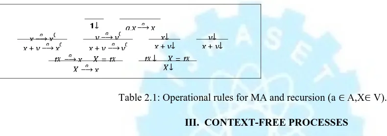
We find that a finite recursive specification over MA can be seen as a rightlinear grammar. Now each finite transition system corresponds directly to a finite recursive specification over MA, using a variable for every state. To go from a term over MA to a transition system, we use structural operational semantics, with rules

Table 2.1: Operational rules for MA and recursion (a ∖A,X∖V).

III. CONTEXT-FREE PROCESSES

Considering the automata theoretic notion of a context-free grammar, we find a correspondence in process theory by taking a recursive specification over a finite set of variables, and over the Sequential Algebra SA, which is MA

Table 3.1: Operational rules for sequential composition (a ∖A).

sequential composition · . We extend the operational rules of Table 2.1 with rules for sequential composition, in Table 3.1. Now consider the following specification

S = 1 + S · a.1.

Our first observation is that, by means of the operational rules, we derive an infinite transition system, which moreover is infinitely branching. All the states of this transition system are different in bisimulation semantics, and so this is in fact an infinitely branching process. Our second observation is that this recursive specification has infinitely many different (non-bisimilar) solutions in the transition system model, since adding any non-terminating branch to the initial node will also give a solution. This is because the equation is unguarded, the right-hand side contains a variable that is not in the scope of an action-prefix operator, and also cannot be brought into such a form. So, if there are multiple solutions to a recursive specification, we have multiple processes that correspond to this specification. This is an undesired property.

These two observations are the reason to restrict to guarded recursive specifications only. It is well-known that a guarded recursive specification has a unique solution in the transition system model. This restriction leads to the following definition.

x−∔xa 0

x·y−∔xa 0_·y x∕ y

a

−∔y0

x·y−a∔y0 x∕_x·yy_∕∕

1∕ _a.x−a_∔x

x−a∔x0

x+y−a∔x0 y

a

−∔y0

x+y−∔a y0 _x+x∕_{y∕ x+}y∕_y∕

tX −∔a x X =tX

X−a∔x t

X∕ X=tX

DEFINITION 4. A context-free process is the bisimulation equivalence class of the transition system generated by a finite guarded recursive specification over Sequential Algebra SA.

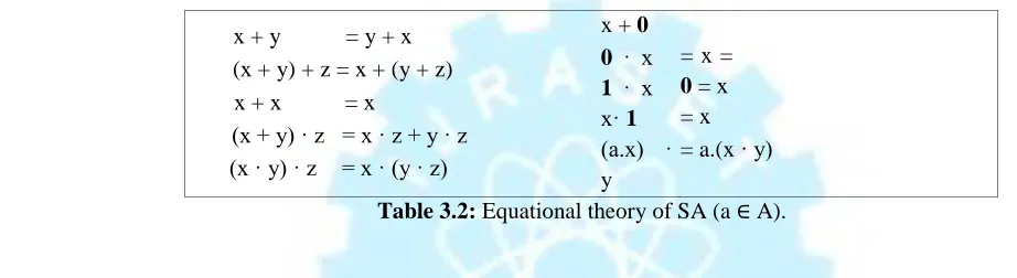
In this paper, we use equational reasoning to manipulate recursive specifications. The equational theory of SA is given in

Table 3.2. Note that the axioms x · (y + z) = x · y + x · z and x · 0 = 0do not hold in bisimulation semantics (in contrast to language equivalence). The given theory constitutes a sound and ground-complete axiomatization of the model of transition systems modulo bisimulation. Furthermore, we often use the aforementioned principle, that guarded recursive specifications have unique solutions [6].

Using the axioms, any guarded recursive specification can be brought into Greibach normal form [4]:

X = X ai.ξi(+ 1).

i∖IX

In this form, every right-hand side of every equation consists of a number of summands, indexed by a finite set IX (the empty sum is 0), each of which is

x + y = y + x (x + y) + z = x + (y + z) x + x = x

(x + y) · z = x · z + y · z (x · y) · z = x · (y · z)

x + 0 0 · x 1 · x

x· 1

(a.x) ·

y

= x = 0 = x = x = a.(x · y)

Table 3.2: Equational theory of SA (a ∖A).

1, or of the form ai.ξi, where ξi is the sequential composition of a number of variables (the empty sequence is 1). We define I as the multiset resulting of the union of all index sets. For a recursive specification in Greibach normal form, every state of the transition system is given by a sequence of variables. Note that we can take the index sets associated with the variables to be disjoint, so that we can define a function V : I → V that gives, for any index that occurs somewhere in the specification, the variable of the equation in which it occurs.

As an example, we consider the important context-free process stack. Suppose D is a finite data set, then we define the following actions in A, for each d∈D:

–?d: push d onto the stack; –!d: pop d from the stack.

Now the recursive specification is as follows:

S = 1 + X ?d.S· !d.S. d∖D

In order to see that the above process indeed defines a stack, define processes Sσ, denoting the stack with contents σ _∈D∗, as

follows: the first equation for the empty stack, the second for any nonempty stack, with top d and tail σ:

Sε= S, Sdσ= S · !d.Sσ.

d∖D e∖D

We obtain the following specification for the stack in Greibach normal form:

S = 1 + X ?d.Td· S, Td = !d.1 + X

?e.Te· Td.

d∖D e∖D

Finally, we define the forgetful stack, which can forget a datum it has received when popped, as follows:

S = 1 + X ?d.S· (1 + !d.S). d∖D

Due to the presence of 1, a context-free process may have unbounded branching [8] that we need to mimic with our pushdown automaton. One possible solution is to use forgetfulness of the stack to get this unbounded branching in our pushdown automaton. Note that when using a more restrictive notion of context-free processes we have bounded branching, and thus we don’t need the forgetfulness property.

The above presented specifications are still meaningful when D is an infinite data set , but does not represent a term in SA anymore. In this paper, we use infinite summation in some intermediate results, but the end results are finite. Note that the infinite sums also preserve THE NOTION OF CONGRUENCE WE ARE WORKING WITH.

Now, consider the notion of a pushdown automaton. A pushdown automaton is just a finite automaton, but at every step it can push a number of elements onto a stack, or it can pop the top of the stack, and take this informationinto account in determining the next move. Thus, making the interaction explicit, a pushdown automaton is a regular process communicating with a stack.

In order to model the interaction between the regular process and the stack, we briefly introduce communication by synchronization. We introduce the Communication Algebra CA, which extends MA and SA with the parallel composition operator k. Parallel processes can execute actions independently (called interleaving), or can synchronize by executing matching actions. In this paper, it is sufficient to use a particular communication function, that will only synchronize actions !d and ?d (for the same d

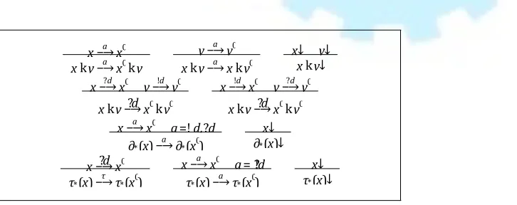
∈D). The result of such a synchronization is denoted ?!d. CA also contains the encapsulation operator ∂∗( ), which blocks actions !d and ?d, and the abstraction operator τ∗( ) which turns all ?!d actions into the internal action τ. We show the operational rules in Table 3.3.

Table 3.3: Operational rules for CA (a ∖A).

Our finite axiomatization of transition systems of CA modulo rooted branching bisimulation uses the auxiliary operators. See Table 3.4 for the axioms and for an explanation of these axioms.T

x−∔a x0

xky−a∔x0_ky y

a

−∔y0

xky−∔a xky0 x∕_xky∕y∕

x−?∔d x0 _y−∔!d _y0

xky−?∔d x0_ky0

x−!∔d x0 _y−?_∔d _y0

xky−?∔d x0_ky0

x−∔a x0 _a=!d,?d

∂∗(x)−∔a ∂∗(x0)

x∕ ∂∗(x)∕

x−?∔d x0 τ∗(x)−τ∔τ∗(x0)

x−a∔x0 a= !?d τ∗(x)−∔a τ∗(x0)

Table 3.4: The given equational theory is sound and ground

bisimulation. This is the preferred model we use, but all our reasoning in the following takes place in the equational theory model-independent provided the models preserve validity of the axioms and unique

[1] Chomsky, Noam. 1962. Context Free Grammar and Pushdown Storage. [2] Waltrous, Ramond L. and Kuhn, Gary M. 1992. Induction of Finite [3] http://www.jflap.org/tutorial/pda/construct/

[4] Context-free grammars and push-down storage [5] N. Chomsky, G.A. MillerFinite state languages

[6] Baeten, J.C.M., Bergstra, J.A., Klop, J.W.: Decidability of bisi 40(3), 653–682 (1993)

[7] Seymour Ginsburg, Sheila A. Greibach and Michael A. Harrison (1967). "Stack Automata and Compiling

x k y

a.xTy

(x + y) | z 1 | 1 a.x| 1 !d.x| ?d.ya.x| b.y

∂∗(0)

∂∗(1)

∂∗(!d.x)

∂∗(a.x)

∂∗(x + y)

= x y + y T

= 0 = 0 = a.(x k y)

= x | z + y | z = 1

= 0

= ?!d.(x k y) = 0 if {a,b}

= 0 = 1

= ∂∗(?d.x) = = a.∂∗(x)

= ∂∗(x) +

Table 3.4: Equational theory of CA (a ∖A ∪{τ}).

The given equational theory is sound and ground-complete for the model of transition systems modulo rooted branching bisimulation. This is the preferred model we use, but all our reasoning in the following takes place in the equational theory

independent provided the models preserve validity of the axioms and unique solutions for guarded recursive specifications.

REFERENCES

Chomsky, Noam. 1962. Context Free Grammar and Pushdown Storage.

Waltrous, Ramond L. and Kuhn, Gary M. 1992. Induction of Finite-State Languages

Baeten, J.C.M., Bergstra, J.A., Klop, J.W.: Decidability of bisimulation equivalence for processes generating context-free languages. Journal of the ACM

Seymour Ginsburg, Sheila A. Greibach and Michael A. Harrison (1967). "Stack Automata and Compiling

y + y x + x | y T

= a.(x k y)

= x | z + y | z

= ?!d.(x k y)

if {a,b} 6= {!d,?d}

(?d.x) = 0

if a 6∖{!d,?d}

(x) + ∂∗(y)

a.(τ.(x + y) +

x | y x k 1 1 | x + 1 (x k y) k z (x | y) | z (x y) z

(x |Ty) Tz x

τ.

yTx |Tτ.y

τ∗(0) τ∗(1)

τ∗(?!d.x)

τ∗(a.x)

τ∗(x + y)

x) = a.(x + y)

= y | x = x = 1

= x k (y k z) = x | (y | z) = x (y k z)

= x T| (y z)

= x y T

= 0 T

= 0 = 1

= τ.τ∗(x)

= a.τ∗(x)

= τ∗(x) + τ∗(y if )

a6= ?!d

transition systems modulo rooted branching bisimulation. This is the preferred model we use, but all our reasoning in the following takes place in the equational theory, so is

solutions for guarded recursive specifications.

free languages. Journal of the ACM