Topics in unsupervised learning

Terms and Conditions of Use of Digitised Theses from Trinity College Library Dublin

Copyright statement

All material supplied by Trinity College Library is protected by copyright (under the Copyright and Related Rights Act, 2000 as amended) and other relevant Intellectual Property Rights. By accessing and using a Digitised Thesis from Trinity College Library you acknowledge that all Intellectual Property Rights in any Works supplied are the sole and exclusive property of the copyright and/or other I PR holder. Specific copyright holders may not be explicitly identified. Use of materials from other sources within a thesis should not be construed as a claim over them.

A non-exclusive, non-transferable licence is hereby granted to those using or reproducing, in whole or in part, the material for valid purposes, providing the copyright owners are acknowledged using the normal conventions. Where specific permission to use material is required, this is identified and such permission must be sought from the copyright holder or agency cited.

Liability statement

By using a Digitised Thesis, I accept that Trinity College Dublin bears no legal responsibility for the accuracy, legality or comprehensiveness of materials contained within the thesis, and that Trinity College Dublin accepts no liability for indirect, consequential, or incidental, damages or losses arising from use of the thesis for whatever reason. Information located in a thesis may be subject to specific use constraints, details of which may not be explicitly described. It is the responsibility of potential and actual users to be aware of such constraints and to abide by them. By making use of material from a digitised thesis, you accept these copyright and disclaimer provisions. Where it is brought to the attention of Trinity College Library that there may be a breach of copyright or other restraint, it is the policy to withdraw or take down access to a thesis while the issue is being resolved.

Access Agreement

By using a Digitised Thesis from Trinity College Library you are bound by the following Terms & Conditions. Please read them carefully.

by

Paul David McNicholas

A thesis subm itted to th e University of D ubhn in satisfaction of the requirem ent for th e degree of

D octor of Philosophy

D epartm ent of Statistics, University of Dublin, Trinity College.

O

This thesis has not been subm itted as an exercise for a degree at this or any other Univer­ sity and it is entirely my own work. I agree th a t the Library may lend or copy this thesis upon request; this permission covers only single copies made for study purposes, subject to normal conditions of acknowledgement. The copyright belongs jointly to the University of Dublin and Paul David McNicholas.

Two topics in unsupervised learning are reviewed and developed; namely, m odel-based clustering and association rule m ining.

A new fam ily of G aussian m ix tu re models, w ith a parsim onious covariance stru c tu re , is introduced. T he m ixtures of factor analysers and m ixtures of principal com ponent analysers m odels are special cases of this new fam ily of models. T his fam ily exhibit th e feature th a t th e ir num ber of covariance p aram eters grows linearly w ith th e dim ensionality of th e d a ta , which leads to relatively fast co m p u tatio n tim e. T hese m odels perform excellently, com pared to po p u lar m odel-based clustering techniques, w hen applied to real d a ta .

A new fam ily of G aussian m ix tu re m odels w ith a Cholesky-decom posed covariance stru c tu re is also introduced. Four m em bers of th is fam ily are developed a n d applied to real d a ta . T his fam ily of m odels has great p o ten tia l for fu rth e r developm ent in fu tu re work.

I gratefully acknowledge the guidance, support and patience of my supervisors, Dr. Bren­ dan M urphy and Dr. M yra O ’Regan. Specifically, to Dr. M urphy for dem onstrating and explaining to me many invaluable research techniques, encouraging me to apply m athem at­ ical reasoning to statistical problems and for giving me trem endous support throughout my tim e as a postgraduate student. Specifically, to Dr. O ’Regan for frequently reminding me to refer both to first principles and the practical applications of my work.

In addition, I would like to thank Prof. John H aslett, Mr. Eamonn Mullins and Ms. Deirdre Toher for their advice on particular aspects of my work. I would like to add a special note of thanks to Mr. Aaron McDaid, Mr. Derrnot Frost and Mr. Michael Salter-Townshend for their generous advice on programming in C.

Thanks to Prof. Patrick Prendergast, Dean of G raduate Studies, and Dr. Mike Peardon, Course Director for the MSc in High Performance Computing, for allowing me to take an MSc in High Performance Com puting while completing this work. The knowledge gained from this course has been valuable while completing some of the research outlined herein, and will be of great benefit in future research.

I would like to extend a very special note of personal gratitude to Prof. Petros Florides, Mr. Eam onn Mullins, Dr. Donal O ’Donovan and Dr. M yra O ’Regan who have each given me fantastic support and encouragement throughout my years at university. Furtherm ore, Ms. Sharon King, Mr. John McCarthy, Mr. Aaron McDaid, Ms. Eimhi'n Nf M huircheartaigh, Mr. S tuart O ’Neill and Mr. Michael Salter-Townshend provided me with great personal support throughout my time as a postgraduate student, for which I am very grateful. I am also grateful to my family for their continued support.

I would like to gratefully acknowledge the contribution of my examiners. Prof. John Hinde and Dr. Krzysztof Mosurski, for their helpful comments and suggestions. Thanks are also due to Ms. Sharon King for translating the variable names from the coffee d ata from German into English.

P u b lication s

The following articles, arising from this work, are to be published or are under review.

McNicholas, P. D., Murphy, T. B. and O ’Regan, M., ‘Standardising the Lift of an As­ sociation Rule’, Computational Statistics and Data Analysis (under review).

McNicholas, P. D. and Murphy, T. B., ‘Parsimonious Gaussian M ixture M odels’, Com­ putational Statistics (conditionally accepted).

C ontents

L ist o f F ig u r e s x iii

L ist o f T a b le s x v

1 I n tr o d u c tio n 1

1.1 Unsupervised L e a rn in g ... 1

1.1.1 D e f in itio n ... 1

1.1.2 Model-Based C lu s te r in g ... 2

1.1.3 Association Rule M in in g ... 2

1.2 Thesis S t r u c t u r e ... 2

1.2.1 C hapter 2 ... 2

1.2.2 C hapter 3 ... 3

1.2.3 C hapter 4 ... 3

1.2.4 C hapter 5 ... 3

1.2.5 C hapter 6 ... 4

1.2.6 C hapter 7 ... 4

1.2.7 C hapter 8 ... 4

1.2.8 C hapter 9 ... 5

1.3 The Im pact of this W o rk ... 5

2 M o d e l- B a s e d C lu s te r in g 7 2.1 B a c k g ro u n d ... 7

2.2 M ixture M o d e ls ... 7

2.2.1 Finite M ixture M o d e ls ... 7

2.2.2 Gaussian M ixture M o d e ls ... 8

2.3 The Expectation-M axim isation A lg o rith m ... 8

2.3.1 MM Algorithms ... 8

2.3.2 The EM A lg o rith m ... 9

2.4 MCLUST: Software for Model-Based Cluster A n a ly s is ... 10

2.5 Variable S electio n... 12

2.6 M ixture Model Selection &: P e rfo rm a n c e ... 12

2.6.1 The Bayesian Information Criterion ... 12

2.6.3 Note on Performance Assessment for Model-Based Clustering . . . . 14

3 P a r s im o n io u s G a u s s ia n M ix tu r e M o d e ls 15 3.1 In tro d u c tio n ... 15

3.2 Factor A n a ly s is ... 15

3.2.1 The Model ... 15

3.2.2 The Likelihood F u n c tio n ... 16

3.2.3 The EM Algorithm for the Factor Analysis M o d e l ... 17

3.2.4 The Probabilistic Principal Component Analysis M o d e l ... 19

3.2.5 M ixtures of Factor Analysers &: M ixtures of Probabilistic Principal Component A n a ly s e r s ... 19

3.3 Parsimonious G aussian M ixture M o d e l s ... 20

3.3.1 Covariance S t r u c t u r e s ... 20

3.3.2 Model F i t t i n g ... 21

3.3.3 L ik e h h o o d s ... 21

3.3.4 The M o d e ls ... 23

3.3.5 Convergence C r ite r ia ... 25

3.3.6 S o ftw are... 26

3.3.7 Model Selection k. P erfo rm an c e... 28

3.4 Coffee D a t a ... 28

3.4.1 The D a t a ... 28

3.4.2 The PGM M Family of Models ... 29

3.4.3 The MCLUST Family of M o d e l s ... 30

3.4.4 Model C o m p a ris o n ... 30

3.5 Italian Wine D ata ... 31

3.5.1 The D a t a ... 31

3.5.2 The PGM M Family of Models ... 31

3.5.3 The MCLUST Family of M o d e l s ... 32

3.5.4 Variable Selection ... 33

3.5.5 Model C o m p a ris o n ... 33

3.5.6 Deeper into the Italian Wine D ataset ... 34

3.6 The Larger Wine D a t a s e t ... 34

3.6.1 The Remaining V a r ia b l e s ... 34

3.6.2 The PGM M Family of Models ... 35

3.6.3 The MCLUST Family of M o d e l s ... 36

3.6.4 Variable Selection ... 36

3.6.5 Model C o m p a ris o n ... 37

3.7 D iscussion... 37

4 G e n e ra lis e d P a r s im o n io u s G a u s s ia n M ix tu r e M o d e ls 39 4.1 S t r u c t u r e ... 39

4.1.1 Redefining ... 39

4.1.2 The Q E q u a t i o n ... 39

4.2 Param eter Estim ates for G P G M M s... 40

4.2.2 M ethod of Lagrange M ultip liers... 41

4.2.3 P aram eter Estim ates for the CCUU Model ... 42

4.3 Leptograpsus Crabs D a t a ... 43

4.3.1 The D a t a ... 43

4.3.2 The GPGM M Family of Models ... 44

4.3.3 The MCLUST Family of Models & Variable S e le c tio n ... 45

4.3.4 Model C o m p a ris o n ... 46

4.4 S u m m a r y ... 47

5 P a r s im o n io u s G a u s s ia n M ix tu r e M o d e ls w ith C h o le s k y -D e c o m p o s e d C o- v a ria n c e S t r u c t u r e 49 5.1 In tro d u c tio n ... 49

5.2 B a c k g ro u n d ... 49

5.2.1 Cholesky D eco m po sition ... 49

5.2.2 Modified Cholesky Decomposition ... 50

5.3 Parsimonious Gaussian Alixture Models with Cholesky-Decomposed Covari­ ance Structure ... 50

5.3.1 The Model ... 50

5.3.2 Model F i t t i n g ... 51

5.3.3 Param eter Estim ates for the VV M o d e l ... 53

5.4 R ats D a t a ... 54

5.4.1 The D a t a ... 54

5.4.2 A n a ly s is ... 55

5.4.3 Results ... 55

5.5 S u m m a r y ... 56

6 A s s o c ia tio n R u le s 59 6.1 In tro d u c tio n ... 59

6.2 Definition of an Association R u l e ... 60

6.2.1 Association R u le s ... 60

6.2.2 N e g a tio n s ... 60

6.3 Support, Confidence, Expected Confidence & L i f t ... 61

6.4 Rule Generation ... 61

6.5 Lift & Odds R a t io s ... 62

6.5.1 The L i f t ... 62

6.5.2 2 x 2 Tables &: Odds R a t i o s ... 63

6.6 Association Rule Visualisation ... 64

6.6.1 Two-Key P l o t s ... 64

6.6.2 Doubledecker P l o t s ... 64

6.7 P r u n i n g ... 67

6.7.1 Test 1 ... 67

6.7.2 Test 2 ... 68

6.7.3 Test 3 ... 68

6.7.4 R e m a r k ... 68

6.8.1 Gray &: Orlowska’s Interestingness... 69

6.8.2 Dong & Li’s Interestingness... 70

7 A sso c ia tio n R u le A n alysis o f CAO D a ta 71 7.1 In tro d u ctio n... 71

7.2 B ack g ro u n d ... 71

7.3 L ite r a tu r e ... 72

7.4 Methodology &: D a t a ... 74

7.4.1 M eth o d o lo g y ... 74

7.4.2 D a t a ... 74

7.5 Analysis of Rules Interrelating C ourses... 76

7.5.1 Rule G e n e ra tio n ... 76

7.5.2 Pruning M e t h o d ... 77

7.5.3 Top Twenty R u l e s ... 78

7.5.4 Remaining R u le s ... 80

7.5.5 R em arks... 81

7.6 Further Exploratory A n a ly sis ... 81

7.6.1 The Idea ... 81

7.6.2 M eth o d o lo g y ... 82

7.6.3 Results ... 82

7.7 Analysis of Gender Related Choices — F e m a l e ... 82

7.7.1 Initial A n a ly sis... 82

7.7.2 An Alternative Approach — Gray & Orlowska’s Interestingness . . . 83

7.7.3 Top Ten R u l e s ... 84

7.7.4 Further R u le s ... 86

7.8 M iscellaneous... 86

7.8.1 Analysis of Gender Related Choices — Male ... 86

7.8.2 Results of Analyses for Alternative Support & Confidence Thresholds 86 7.9 C onclusions... 87

7.9.1 A Word of Warning ... 87

8 S ta n d a rd is in g th e Lift of a n A ssociation R ule 89 8.1 Introdu ction... 89

8.2 Range of Values of L if t... 90

8.2.1 Range in Terms of P{A) & P { B )... 90

8.2.2 Range in Terms of the Minimum Support Threshold or the Number of T ran sactio n s... 90

8.2.3 Range in Terms of P{A), P{B), Support &: Confidence Thresholds . 91 8.2.4 Standardisation... 91

8.3 Example I: College Application D a t a ... 92

8.3.1 Background & D a t a ... 92

8.3.2 Initial A n a ly sis... 92

8.3.3 Analysis of Rules with Consequent ‘Female’ ... 94

8.3.4 R e m a r k ... 96

8.4.1 The D a t a ... 96

8.4.2 Negations &: C o d i n g ... 97

8.4.3 Resulting R u le s ... 98

8.4.4 Results ... 98

8.5 N e g a tio n s ... 99

8.5.1 Background — Negative Association R u l e s ... 99

8.5.2 How Many More R u le s ... 99

8.5.3 Mining Association Rules Involving N egations... 100

8.6 S u m m a r y ... 101

9 C o n c lu sio n s 103 9.1 S u m m a r y ... 103

9.1.1 Model-Based C lu s te r in g ... 103

9.1.2 Association Rule M in in g ... 104

9.2 Further W o r k ... 104

9.2.1 Modelling the Mean in Model-Based C lu s te rin g ... 104

9.2.2 Allowing the Number of Factors to Vary Across G r o u p s ... 105

9.2.3 Application of Generalised Procrustes Analysis to Model-Based Clus­ tering ... 105

9.2.4 P arallelisatio n ... 105

9.2.5 Further Expansion of the CDGMM F a m i l y ... 106

9.2.6 Model Selection & Convergence C r i t e r i a ... 106

9.2.7 Association R u le s ... 106

9.2.8 The CAO D a t a ... 106

A C a lc u la tio n s fo r P G M M s 119 A .l Im portant Results ... 119

A.2 Q E q u a t i o n ... 120

A.3 Differentiation ... 120

A.4 Maximum Likelihood E s tim a te s ... 121

A.4.1 Model C C C ... 121

A.4.2 Model C C U ... 121

A.4.3 Model C U C ... 122

A.4.4 Model C U U ... 123

A.4.5 Model U C C ... 124

A.4.6 Model U C U ... 124

A.4.7 Model U U C ... 125

A.4.8 Model U U U ... 125

B C a lc u la tio n s fo r G P G M M s 127 B .l Im portant Results ... 127

B.2 Q E q u a t i o n ... 127

B.3 Constrained Maximum Likelihood Estim ates ... 128

B.3.1 Model U C U U ... 128

B.3.3 Model U U C U ... 130

C C a lc u la tio n s fo r C D G M M s 133 C .l Q E q u a t i o n ... 133

C.2 Maximum Likeliliood E s tim a te s ... 133

C.2.1 Model V E ... 133

C.2.2 Model E V ... 134

C.2.3 Model E E ... 136

D C o d in g 137 D .l B a c k g ro u n d ... 137

D.2 F u n c tio n a lity ... 137

D.2.1 Organisation &: Input ... 137

D.2.2 Command L i n e ... 138

D.2.3 O utput to F i l e s ... 138

D.2.4 O utput to S c re e n ... 139

D.2.5 Notes on the Structure of the C o d e ... 139

D.2.6 Example of an AECM A lg o rith m ... 141

D.2.7 Com patibility of O utput with R ... 143

E T ab les fro m th e A n a ly s is o f C A O D a ta 145 E .l Explanation of Course C o d e s ... 145

E.2 Rules Interrelating Courses ... 148

E.3 Rules with Consequent { F }... 150

E.4 Rules with Consequent { M }... 151

F L ift &; N e g a tio n s 153 F .l Range of Values for L i f t ... 153

List o f F igu res

2.1 Cluster shapes th a t correspond to the covariance structures given in Table 2.1. 11

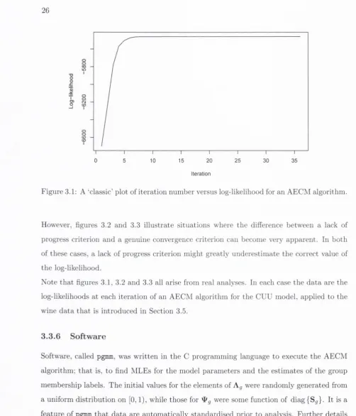
3.1 A ‘classic’ plot of iteration number versus log-likelihood for an AECM algo­

rith m ... 26

3.2 A plot of iteration number versus log-likelihood for an AECM algorithm, illustrating a single ‘step ’... 27

3.3 A plot of iteration number versus log-likelihood for an AECM algorithm, illustrating multiple ‘steps’... 27

3.4 A ‘heat m ap’ giving the maximum BIC value for each PGMM at (G, q) for the coffee d a ta ... 29

3.5 A ‘heat m ap ’ giving the greatest BIC values for each PGM M at {G,q) for the wine d ata from g c lu s ... 32

3.6 A ‘heat m ap’ giving the greatest BIC values for each PGM M at {G, q) for the larger wine d ataset... 35

4.1 A ‘heat m ap’ giving the greatest BIC values for each GPGM M at {G,q) for the crabs d a ta ... 45

4.2 A pairs plot of the crabs data, constructed using R ... 46

5.1 Time series for each rat, coloured by group — black for rats from Diet 1, red for Diet 2 and green for Diet 3... 55

5.2 Time series for each rat, coloured by classifications — black for Group 1, red for Group 2, green for G roup 3, purple for Group 4 and blue for Group 5. . 56

6.1 An example of a two-key p lo t... 65

6.2 A two-key plot with a rectangle enclosing all rules with confidence of at least 0.6 and support of at least 0.4... 65

6.3 Doubledecker plot arising from the rule A ^ B... 66

6.4 Doubledecker plot arising from the rule {A, B } => {C, D }... 67

7.1 The ten most popular course choices in the year 2000... 75

7.2 The ten most popular first preference course choices in the year 2000. . . . 76

8.1 The lift of the rules in Table 8.2 with upper (w) and lower (A) bounds. . . . 93 8.2 The hft of the rules in Table 8.2 with upper (t>) and lower (A*) bounds. . . 93 8.3 The lift of the rules in Table 8.4 with upper {v) and lower (A*) bounds. . . 95 8.4 The number of ‘yes’ answers given to each question by the sample of surveyed

Germans... 97 8.5 The lift of the ten rules, given in Table 8.7, along with their upper {v) and

List o f Tables

2.1 A variety of covariance stru ctu res, S g , available using m c lu s t, along w ith th e num ber of covariance param eters in each case... 11

3.1 T he covariance stru c tu re and num ber of covariance p aram eters for each PG M M . 20 3.2 Twelve of th e th irte e n chemical p roperties of coffee given by Streuli (1973). 29 3.3 Classification tab le for the best PG M M for th e coffee d a ta ... 30 3.4 Classification tab le for th e best M C LU ST m odel for th e coffee d a ta ... 30 3.5 R an d an d a d ju sted R and indices for b o th families of m odels th a t were applied

to th e coffee d a ta ... 30 3.6 T h e th irte e n chem ical properties of wine, used by Forina et al. (1986), th a t

are available in gclus... 31 3.7 Classification tab le for th e best PG M M for th e wine d a ta from g c lu s . . . . 31 3.8 Classification tab le for th e best M C LU ST m odel for th e wine d a ta from g c lu s . 32 3.9 Classification tab le for variable selection for th e wine d a ta from g lu s . . . . 33 3.10 R an d and a d ju sted R and indices for all of m odels th a t were applied to th e

wine d a ta from g c l u s ... 33 3.11 T h e wine d a ta from g c lu s ordered by year of p ro d u c tio n ... 34 3.12 Classification tab le for th e best PG M M m odel for th e wine d a ta from g c lu s ,

ordered by y e ar... 34 3.13 T he fifteen chemical properties of wine, used by Forina et al. (1986), th a t

were not available in gclus... 35 3.14 C lassification tab le for th e best PG M M for th e larger wine d a ta s e t... 36 3.15 C lassification tab le for the best M CLU ST m odel for th e larger wine d a ta se t. 36 3.16 V ariables selected for th e larger wine d a ta s e t... 36 3.17 Classification tab le for variable selection on th e larger wine d a ta s e t... 37 3.18 R a n d and a d ju ste d R and indices for all m odels applied to th e larger wine

d a ta s e t... 37

4.5 Classification table from the MCLUST analysis of the crabs d ata... 45

4.6 Classification table from the variable selection analysis of the crabs data. . 46

4.7 Rand and adjusted Rand indices and error rate for all of the models th at were applied to the crabs d a ta ... 47

5.1 The covariance structure and number of covariance parameters for each CDGMM... 51

5.2 Classification table for the best CDGMM on the rats dataset... 55

6.1 Common functions of association rules... 61

6.2 A cross-tabulation of A versus B... 63

7.1 The top twenty rules, ranked by confidence, interrelating courses... 79

7.2 The top ten rules, ranked by confidence, with consequent {F}... 83

7.3 The top ten rules, ranked by interestingness, with consequent {F}... 83

7.4 Gender breakdown of primary teaching staff’ in Ireland, 1999-2004... 85

8.1 The four mined rules that contained only medicine courses... 92

8.2 The four rules from Table 8.1, with their bounds for lift... 92

8.3 Standardised lifts for the four rules listed in Table 8.1... 94

8.4 The highest ranked, by Int(A => B ;2,2), rules with consequent { F}... 95

8.5 Standardised lift for the three highest ranked rules with consequent {i^}. . 95

8.6 The questions th at were asked in the German ‘social life feeling’ study. . . . 96

8.7 Top ten rules from the German ‘social life feeling’ data, ranked by £*. . . . 98

D .l The command line options available in pgmm... 138

D.2 The files produced by running pgmm... 139

E .l Course codes appearing in this work... 145

E.2 The 72 rules mentioned in Section 7.5.4, ranked by confidence... 148

E.3 Top twenty rules, ranked by interestingness, with consequent {F}... 150

C hapter 1

Introduction

1.1

U n su p er v ise d L earning

1.1.1 D e fin it io n

H astie et al. (2001) give th e analogy of “learning w ithout a teach er” when introducing unsupervised learning. Formally, th ey consider a set of n realisations { x \ , x2, ■■. ,x „ } of a random p-dim ensional vector x w ith jo in t p robability d istrib u tio n P (x ). T he objective is th en to deduce pro p erties of P (x ) w ith o u t knowing th e correct answers, th a t is “w ithout th e help of a supervisor” .

T his approach to s ta tistic a l learning can also be distinguished by w hether or not th e o u t­ come, or ta rg e t, variable is present in th e learning process. A m odel learns in a supervised fashion when th e outcom e variable is present during th e learning process, while in th e un­ supervised learning context, th e outcom e variable is either missing, non-existent or th ere is no obvious outcom e variable.

1 .1 .2 M o d e l-B a se d C lu ste r in g

Clustering based on m ixture models has appeared in the literature with increased frequency in recent years. The approach followed herein involves a family of Gaussian m ixture models w ith parsimonious covariance structure. The clustering of the data, according to this family of models, is given by the values assigned to the group membership labels through the learning process. Well-established m ixture modelling techniques are used for motivation and the m athem atical foundation of this family of models is established. These models are then applied to real d ata and perform favorably when compared to well-established techniques. A family of Gaussian m ixture models th a t can be applied to longitudinal d ata is also introduced.

1 .1 .3 A ss o c ia tio n R u le M in in g

Association rule mining is developed as an effective m ethod of analysing binary data. A novel application of association rules to a ‘clustering’ problem is dem onstrated and a method of standardising the lift of an association rule is introduced th a t leads to a new measure of interestingness. Additionally, the num ber of potentially interesting association rules th a t can be mined from a binary d ataset is quantified and an argum ent is put forward for the inclusion of negations in association rule analysis.

1.2

T h esis S tru ctu re

1.2 .1 C h a p ter 2

1.2.2

C hapter 3

P arsim onious G aussian m ixture m odels are developed using a late n t G aussian m odel which is closely related to th e factor analysis model. T hese m odels provide a unified m odelling fram ew ork which includes th e m ixtures of factor of analysers and m ixtures of probabilistic principal com ponent analysers m odels as special cases. In p a rticu la r, a class of eight p a r­ sim onious G aussian m ix tu re models, which are based on th e m ixtures of factor analysers m odel, are introduced.

A m ethod for o b taining th e m axim um likelihood estim ates for th e p aram eters in these m odels, via an A ECM algorithm , is d em o n stra ted . T his fam ily of m odels includes five parsim onious m odels th a t have not previously been developed. All m em bers of this family have th e a ttra c tiv e p ro p erty th a t th eir num ber of covariance p aram eters is linear in th e dim ensionality of th e d a ta . These m odels are applied to th e analysis of chem ical and physical properties of Italian wines and th e chem ical p roperties of coffee; th e m odels are shown to give superior clustering results w hen com pared to w ell-established techniques.

1.2.3

C hapter 4

C h a p te r 4 builds on th e ideas in C h a p te r 3 w ith th e covariance stru c tu re of th e m ixture m odels being fu rth e r generalised. T his results in four e x tra models. These m odels also have a num ber of covariance p aram eters th a t is linear in the dim ensionality of th e d a ta . None of these four m odels have previously ap p eared in th e lite ra tu re and com bined w ith th e eight m odels from C h a p te r 3, th ey give a fam ily of twelve parsim onious G aussian m ix tu re models. T hese m odels are applied to crabs d a ta w here th ey give excellent results when com pared to w ell-established techniques.

1.2.4

C hapter 5

models is shown to perform well when applied to real data. Further developments of this covariance structure, th a t could potentially increase the number of models in this family, are also suggested.

1 .2 .5 C h a p ter 6

This chapter marks the change in emphasis from interval d ata to binary d ata and thus the switch from model-based clustering to association rule mining. In C hapter 6 association rules are introduced. The term ‘association rule’ is defined, along with related functions, and the popular literature is summarised. Various m ethods of generating, pruning and ranking rules are introduced and reviewed.

1 .2 .6 C h a p ter 7

C hapter 7 introduces the novel idea of using association rules to reveal grouping in data. Central Applications Office college application d a ta is analysed using association rule mining to investigate relationships between course choices across applicants. The role of gender as a factor in course selection is examined as well as a larger question around the functionality of the application system — w hat a ttra c ts students to a course; is it a topic of interest or is it the perceived status of the course associated with high entry points?

The expected gender imbalances in areas like prim ary teaching and engineering appear, along with some others. Association rules generated suggest th a t students select courses based prim arily on topic but sometimes with geographical location in mind. No evidence is found to suggest th a t students are selecting courses based on perceived points status.

1 .2 .7 C h a p ter 8

college application d ata th a t was analysed in C hapter 7 and on German social data. In the la tter case, negations are introduced into the mining paradigm and an argum ent for their inclusion is put forward. This argum ent includes a quantification of the number of extra rules th a t arise when negations are considered.

1.2.8

C hapter 9

The ideas and methods dem onstrated in this work are summarised in C hapter 9. Suggestions for further work are given, both based upon and arising from this work.

1.3

T h e Im p act o f th is W ork

The im pact of this work on the body of literature is summarised here based on the most significant original ideas contained herein. The principal novel features of this work are:

• A new family of Gaussian m ixture models, with a parsimonious covariance structure, is introduced. The covariance structure is similar to th a t of the m ixtures of factor analysers model, which is in fact a member of this family. This new family of models exhibit the feature th a t their number of covariance param eters grows linearly with the dimensionality of the data, which leads to relatively fast com putation time. These models perform excellently, compared to popular model-based clustering techniques, when applied to real data.

• A new family of Gaussian m ixture models with a Cholesky-decomposed covariance structure is introduced. Four members of this family are developed and applied to real data. This family of models has great potential for further development in future work.

• A new approach is taken to the analysis of college applications d ata th a t contributes to the discussion about the existence of a ‘points race’.

C h ap ter 2

M odel-B ased C lustering

2.1

B ack grou n d

C h ap ters 3, 4 and 5 of th is work focus on fam ihes of m ix tu re m odels. Each of these families is applied to interval d a ta as a m odel-based clustering technique.

2.2

M ix tu r e M o d els

2.2.1

F in ite M ix tu re M odels

M odel-based clustering techniques can be tra c ed a t least as far back as Wolfe (1963). In m ore recent years m odel-based clustering has ap peared in th e sta tistic s litera tu re w ith increased frequency (Fraley &: R aftery, 1998; M cLachlan et a i , 2003; R aftery h Dean, 2006). T ypically th e d a ta are clustered using some assum ed m ix tu re m odelling stru c tu re and th e p a ra m ete rs associated w ith these m odels are usually e stim ated using an expectation- m axim isation (EM ) algorithm .

ties. Extensive reviews of finite m ix tu re m odels are contained in T itte rin g to n et al. (1985), M cLachlan & Basford (1988) a n d M cLachlan & Peel (2000a).

2.2.2

Gaussian M ix tu r e M odels

T h e G aussian m ixture m odel has received p a rtic u la r a tte n tio n , b o th in th e th re e afore­ m entioned tex ts and in th e w ider body of sta tistic a l literatu re. A G aussian m odel is assum ed for each sub-population, or group. T he m odel density is of th e form

G

/ ( ^ ) = (2 -1 )

5 = 1 where

0(x I

= - ^ = y = = e x p | - ^ ( x - A i g ) ' S - i ( x - / X g ) |

is th e density of a m u ltiv ariate G aussian w ith m ean fig and covariance S g , and Hg is the probability of m em bership of group g. A review of G aussian m ixture m odels w ith p a rticu la r em phasis on applications to clu ster analysis, discrim inant analysis an d density estim ation is given by Fraley & R aftery (20026).

2.3

T h e E x p e c ta tio n -M a x im isa tio n A lg o r ith m

T h e EM algorithm is an ite rativ e m ethod for finding th e m axim um of th e expected value of th e co m p lete-d ata log-likelihood. Before introducing th e EM algorithm , a larger class of algorithm s to which th e EM algorithm belongs is introduced.

2.3.1

M M A lgorithm s

MM algorithm s are a b lueprint for a broad, ever-expanding, class of algorithm s. A review of M M algorithm s is given by H u n ter & Lange (2004) and th e rem ainder of th is section essentially presents a sum m ary of th eir work.

th e MM principle can be seen in th e litera tu re a t least as far back as O rteg a &: R heinboldt (1970) b u t th e first use of th e term MM cam e in H u nter &: Lange (2000).

Let be a fixed value of a p a ra m ete r ip and let g{-) and /( • ) be real-valued functions. T h en g {ip \ is said to m ajorize f { i p) a t th e point if

g{ip I > f { i p) for all <^, and

F urtherm ore, g {ip \ is said to m inorize f { i p) at if —g {ip \ m ajorizes —f { p ) a t <p^^\

F u rth e r details, including th e casting of th e EM algorithm as a special case, are given by H unter & Lange (2004). In th e case of th e EM algorithm , th e m inorising function is th e expected value of th e co m p lete-d ata log-likelihood.

2 .3 .2 T h e E M A lg o r ith m

T h e EM algorithm (D em pster e t al., 1977) provides an iterativ e m eth o d of finding m axim um likelihood estim ates (M LEs) where th e d a ta is incom plete or some of th e d a ta is missing. Im p o rtan tly , th e d a ta does not actually need to be incom plete b u t fram ing problem s as incom plete d a ta problem s often leads to efficient solutions v ia th e EM algorithm .

In th e E -step, th e expected value of th e log-likelihood is com puted based on th e cu rren t estim ates of th e m odel p aram eters and th e ‘co m p le te -d ata ’ vector — th a t is, th e vector of observed d a ta plus m issing d a ta . T his function, th e expected value of th e co m p lete-d ata log-likelihood, is a m inorising function — a fact which follows from Je n se n ’s inequality (Jensen, 1906). In th e M -step, this expected value is m axim ised w ith respect to th e m odel param eters.

2,4

M C L U ST : Softw are for M o d e l-B a se d C lu ster A n a ly sis

T h e general G aussian m ix tu re m odel, given in E q u a tio n 2.1, has a to ta l of

{G — 1) + Gp + Gp{p + l ) / 2

param eters, of which Gp{p + l ) / 2 are from th e group covariance m atrices S g. A sim pler form of th e m ix tu re assum es t h a t th e covariances are constrained to be equal across groups, which reduces to a to ta l of (G — 1) + Gp + p{p + l ) / 2 param eters, of which p{p + l ) / 2 are from th e com m on group covariance m atrix Eg — S .

Banfield &: R aftery (1993), Celeux & G ovaert (1995) a n d Fraley & R aftery (1998, 20026) exploit an eigenvalue decom position of th e group covariance m atrices to give a wide range of covariance stru c tu re s th a t use betw een one and G p { p + l ) / 2 p aram eters. T he eigenvalue decom position of th e covariance m atrix is of th e form

Eg = AgDgAgO;, (2.2)

where Xg is a co n stan t, Dg is a m atrix consisting of th e eigenvectors of Eg and Ag is a diagonal m atrix w ith entries pro p o rtio n al to th e eigenvalues of Eg.

T he m odel-based clustering techniques th a t have been developed using th e covariance stru c ­ tu re given in E q u atio n 2.2 allow for a variety of co n straints. T here is th e option to constrain th e com ponents of th e eigenvalue decom position of Eg across groups of th e m ix tu re model. F urtherm ore, th e m atrices Dg or Dg and Ag m ay be set equal to I, or not.

Fraley & R aftery (2002a, 2003) describe th e m c lu s t software, which is available as a library in th e softw are package R (R D evelopm ent Core Team , 2006). T h e m c lu s t softw are allows efficient m odel-based clustering a n d incorporates th e work of Fraley & R aftery (1998, 1999, 20026). Table 2.1, which is tak e n from D ean et al. (2006), gives th e covariance decom posi­ tio n s th a t are available using th e m c lu s t software. Figure 2.1, w hich is sim ilar to a figure in D ean et al. (2006), provides an illu stratio n of these covariance decom positions.

Table 2.1: A variety of covariance structures, Sg, available using m clu st, along with the number of covariance param eters in each case.

ID Volume Shape O rientation Covariance Decomp.

Number of Covariance Param eters

E li Equal Spherical — AI 1

VII Variable Spherical — Afcl G

EEI Equal Equal Axis-aligned AA _P

VEI Variable Equal Axis-aligned A,A p + G - 1

EVI Equal Variable Axis-aligned AA, pG — G -f-1

VVI Variable Variable Axis-aligned Ag Ag pG

EEE Equal Equal Equal ADAD' p{p + l ) ! 2

EEV Equal Equal Variable

_ADfcADjt

G p { p + l ) / 2 - { G - \ ) p VEV Variable Equal Variable AfcDfcAD'^ G p ( p + l ) / 2 - ( G - l ) ( p - l )

vvv

Variable Variable Variable AfcDfcAfcD^ G p { p + l ) / 2

c >

A

O

o

o °

\J

4

)<

3

^

Figure 2.1: Cluster shapes th a t correspond to the covariance structures given in Table 2.1.

Notably, the number of covariance param eters given in Table 2.1 for the m c lu st models are

either constant, linear or quadratic in p. Therefore, not all of these models are well suited to modelling high dimensional data. In particular, fitting a m ixture model w ith any of

the more general covariance structures available in m c lu st, th a t is the last four covariance

structures given in Table 2.1, to high-dimensional d ata will be extremely com putationally

2.5

V ariable S elec tio n

Raftery & Dean (2006) propose a variable selection method based on the use of Bayes factors. Their approach is that which would be taken to a model selection problem. Two models, Mi and M2 say, for data X are compared using the using Bayes factors. The Bayes factor, Bi2, for model Mi versus model M2, is defined as

p { X I M l ) p { X \ M 2 Y where

p { X I Mfc) = I p { X i dk, Mk)p{ek I Mk)dOk,

Ok is the vector of parameters for model M^ and p{9k \ M^) is the prior distribution of (Kass &: Raftery, 1995). Variables are then selected based on which model is the ‘best’. Variable selection can be carried out using the c lu s t v a r s e l package (Dean Sz Raftery, 2006) in R. The user only needs to preset the maximum number of groups and c lu s t v a r s e l auto­ matically selects the variables. However, due to its nature, variable selection involves many runs of m clust and once the variables are selected the user needs to run m clust on the chosen variables to get the classifications. Therefore, this method has even greater limita­ tions, in terms of computation time, than m clust, and thus will be particularly apparent in applications to high-dimensional data.

2.6

M ix tu re M o d el S e lec tio n

8

^

P erform an ce

2.6.1

T h e B ayesian Inform ation C riterion

The Bayesian information criterion (BIC) (Schwartz, 1978) is often used to select an ap­ propriate mixture model; in the case of m clust, for example. For a model with parameters $ , the BIC is given by

BIC = 2/(x, i ) — m logn ,

be m o tivated th ro u g h an asy m p to tic approxim ation of th e log p osterior probability of the m odels (Kass & R aftery, 1995).

T h e usual regularity conditions for th e asym ptotic approxim ation used in th e developm ent of th e BIC are not generally satisfied by m ixture models. However, Leroux (1992) showed th a t th e BIC, asym ptotically, does not u n d erestim ate th e tru e num ber of m ixture com ponents and K eribin (1998, 2000) showed th a t th e BIC gives consistent estim ates of th e num ber of com ponents in a m ix tu re m odel. F urtherm ore, Fraley k. R aftery (1998, 20026) provide p ractical evidence th a t B IC perform s well as a m odel selection criterion for m ix tu re models. N ote th a t there are altern ativ es to th e B IC for m ix tu re m odel selection; for exam ple, the in teg rated com pleted likelihood (Biernacki et a i, 2000) penalises th e BIC by su b tra c tin g th e estim a ted m ean entropy. However, th e viability of such altern ativ es is not discussed herein and th e BIC alone is used for m odel selection.

2 .6 .2 T h e R a n d &: A d ju ste d R a n d In d ices

T h e perform ance of m ixture m odels in revealing group s tru c tu re in d a ta can m easured using the R and index (R and, 1971) and th e ad ju sted R an d index (H u b ert & A rabie, 1985). T hese indices are com puted on a cross-tabulation of th e m axim um a posteriori (M A P) classification of th e observations w ith th e tru e group m em bership. T he ran d index can be expressed as

num ber of agreem ents

num ber of agreem ents + num ber of disagreem ents ’

w here th e ‘num ber of agreem en ts’ is com puted based on pair agreem ent and th e ‘num ber of disagreem ents’ is based on pair disagreem ent. C onsider an exam ple sim ilar to th a t given by R and (1971), w here a variable w ith two groups y — {{a, b), (c, d, e)} is classified by y = {(a, b, c), {d, e)}. Now, th e num ber of agreem ents is th e num ber of pairs th a t are together in b o th y and y plus th e num ber of pairs th a t are se p ara te in b o th y and y. Therefore, th ere are six agreem ents; ab, de, ad, ae, bd and be. T h e den o m in ato r of E q u atio n 2.3 can be easily com puted as

T h e a d ju ste d R an d index corrects th e R and index for chance by accounting for th e fact th a t

if classification is perform ed random ly some cases will be correctly classified by chance. T h e

indices each take values in [0,1] w ith ‘0 ’ indicating th a t th e M A P classification and tru e

groups never agree and ‘1’ indicating th a t th e th ey are exactly th e same. Large values of

these indices indicate stro n g agreem ent betw een th e tru e groupings and th e classifications

proposed by th e m ixture model.

N ote t h a t th e possibility of using a lte rn a tiv e or additional m easures of class agreem ent, such

as C o h en ’s kappa (Cohen, 1960), was considered b u t th e R and a n d a d ju ste d R an d indices

were th o u g h t to be sufficient for use in th is work.

2.6.3

N o te on Perform ance A ssessm en t for M od el-B ased C lu sterin g

A lthough th e m odel-based clustering techniques described herein are unsupervised, th eir

perform ance is assessed via application to real d a ta and subsequent com parison of th e resulting classifications to th e tru e groups. However, in m any applications th e tru e group

stru c tu re would not be known, which is reflected in the use of th e BIC for m odel selection

Chapter 3

P arsim onious G aussian M ixtu re

M odels

3.1

In tr o d u ctio n

A new family of finite m ixture models is introduced, with a Gaussian model used to model each m ixture component. These m ixture components have a parsimonious factor analysis- Uke covariance structure. The factor analysis and probabilistic principal component analysis models are used for motivation. Crucially, the members of this new family of m ixture models each have a number of covariance param eters th a t grows linearly in the dimensionality of the data.

3.2

Factor A n a ly sis

3.2.1

T h e M od el

factors u, where q ^ p. T he m odel m ay be expressed in the form

/ A n A,, . .. \

x i X2

+ A 2 I A22 ^2q

Ul

U2 €2

\

Xp y

y

y

y Api Ap2 • • •

^pq

/ \

/

\ /

or

X = fj, + A u + e, (3.1)

where A is a p x 9 m atrix o f factor loadings, th e factors u ~ A^(0, Ig) and e ~ A'^(0, where = diag(?/;i, ip2, . . . , ^p). It is a feature o f th e factor analysis m odel th a t A is not uniquely defined; if A is replaced by A* = A D , where D is orthonorm al, then

A A ' + 'I' = (A *)(A " )' + ^ ,

which allows th e results of factor analyses to be rotated, altering their interpretation. This is a large part of th e reason why factor analysis has spent much tim e as “th e black sheep o f sta tistica l theory” (L aw ley k. M axw ell, 1962).

3 .2 .2 T h e L ik elih o o d F u n c tio n

(3.2) From Equation 3.1, th e the d en sity of an Xj is

/ ( x , ! ^ - e x p | - ^ ( x i - ^ ) ' ( A A ' + ^ ') - * ( x , - ^ ) |

s /{2n)P I A A ' + ^ \ [ 2 J

and it follows th a t th e log-likelihood o f x = ( x i , x2, . . . ,x „ ) ' is given by n

/(^, A , ^ ) = ^ l o g / ( x j I

i= l

= - ^ l o g 2 7 T - ^ l o g |A A ' + ^ - /i)

i=l np

log27T — ^ log |A A ' + tr {S(A A ^ + ^') ,

w here S = ( 1 /n ) ~ M )(xi — fi)'- N o te th a t th e d ata on ly appears in th e m odel through S and th a t since th e m atrix ^ is diagonal, th e p x p m atrix (A A ' + ^ ) can be inverted using th e formula

(A A ' + 4 ')-^ = - ^ “ ^A(Ig + (3.4)

(McLachlan & Peel, 2000a), which leaves only q x q matrices to be inverted. McLachlan &

Peel (2000a) also give a convenient formula for finding the determinant of this matrix;

time.

Now, the MLE of is easily obtained by differentiating Equation 3.3 with respect to fx and

setting the result equal to zero to get /x = x. In order to obtain the MLEs of A and an EM algorithm is used.

3 .2 .3 T h e E M A lg o r ith m for th e F actor A n a ly sis M o d e l

E-step

The vector x is taken as the observed data and u as the missing data. The complete-data consist of (x, u); the observed data and the missing data. Before computing the complete- data log-likelihood Id/J-, A , ' ^ ) = lo g /( x , u), it is necessary to compute l o g /( x j | u j ;

I A A ' + ^ 1 = 1 I / I Ip - A' ( A A ' + ^ A (3.5)

The formulae given in equations 3.4 and 3.5 have the potential to greatly reduce computation

- ^ t r { A ' ^ ^ ^ A u , u ' } .

Now,

71

= l o g / ( x , u ) = ^ l o g / ( X i i U , ) / ( U ; )

C - I log l^'l - ^ tr I ^ ^ ^ ( x ; - /i)(x i - ^ )' I + ^ ( x j - /x )'^ ^Auj i=l

n ) n

where C is constant with respect to /x, A, and Now, the expected value of Uj, conditional on Xj and the current model param eters, is

E[uj|xi, /X, A, = A'(AA' + (xj - /x) = /3(xi - ^),

where /3 = A'(AA' + '1')“ ^ = A'S~^, and the expected value of u ,u' conditional on x^ and the current model parameters is

E[UjU'|Xj,/i, A, «»] = Iq - / 3 A + /3(x, - /x)(x; - /x)'/3'.

To complete the E-step, the expected value of the complete-data log-likelihood, which shall be denoted Q(A, ^ ) , is computed at = x.

Q(A, = C - | l o g | ^ j - ^ t r | ^ “ ^ ^ ( x i - A ) '|

" - - i f " - - 1

- l - ^ ( x i - /i) '^ '“ ^AE[uj|xi,/x, A,4'] - ;^tr< A ^ E[u,u' |x,,/i. A, 4'] i

i = \ “

I

i = i

J

= C - ^ log j^'l - ^ tr ^ ( X i - /i)(Xi - A ) '|

-t- tr | ^ ' “ ^ A ^ ^ ( x i - A)(xj - / i ) ' | - ^ tr{ A '« '“ ^A(Ig - 0 A ) }

t ( r n

tr A '^ - ^ A

i=l n

= C + ^ l o g l ’I'-^ l - | t r { ^ “ iS } + n t r { ^ '- iA ;3 S } - | tr{ A '^ “ ^ A © },

where © = Ig — 0 A + /9S/3 is a symmetric q x q m atrix. Although © was introduced as a notational convenience it could be used to devise a model diagnostic, since if S = S then

© = I₉

-M - s te p

(1996) and M agnus & N eudecker (1999) gives

Sl(A,*P) = f x

= n ( < p - ' ) ' ( / 3 S ) ' - ^ | ^ t r { A 0 A ' « I . - ' }

= ^ [ ( 'I '- I ) 'a © ' + A©]

= n « ' " i S ^ ' - n ^ ' “ ^ A 0 .

Now, solving th e equation 5 i(A , ^ ) = 0 gives A = S/9 0 “ ^. D ifferentiating Q w ith respect

to gives,

^ ^ (A')'(A0)'

= | » - ^ S ' + n A 5 S - | A 0 ' A ' .

Now, solving d iag{52(A , 4 ')} — 0 gives

= d i a g j ^ S ' - n A 0 S + ^ A 0 ' [ S ^ ' 0 “ ^ ] '|

=» ^ = d ia g { S ' - 2 A ^ S + = diag {S - A ^ S } .

T he m atrix results used in th is ch ap ter are listed in A ppendix A .I. N ote th a t all m atrices and vectors herein are real, all objects th a t are differentiated are continuously differentiable and th a t all differentials are well defined.

3.2.4

T h e P ro b a b ilistic P rincipal C om p on en t A n alysis M odel

T he probabilistic principal com ponent analysis (P P C A ) m odel (T ipping & B ishop, 19996)

is a special case of th e factor analysis m odel w ith ^ = iplp.

3.2.5

M ixtu res o f Factor A n alysers

M ixtures o f P ro b a b ilistic P rin cip al

C om p on en t A n alysers

Developing th e factor analysis model, G h ah ram an i k. H inton (1997) develop a m ix tu re of

factor analysers m odel, which is fu rth e r developed by M cLachlan &: Peel (2000a). T he density of an observation in group is as in E q u atio n 3.2 w ith = /x^, A = A^ and

analysers tra d itio n ally differ in w hether th e term is constrained to be equal in different groups or not. T ipping & Bishop (1999o) develop th e P P C A m odel to get a m ixture of probabilistic principal com ponent analysers m odel, which is a special case of th e m ixtures of factor analysers model.

3.3

Parsim onious G aussian M ixture M odels

3.3.1

C ovariance S tructures

T h e m odels m entioned in Section 3.2.5 can be extended to a wider fam ily of m odels by constraining, or not,

Ag

=

A,

and w hether ^ g is isotropic. T h e m atrix is said to be isotropic if '^g = tpglp. T he option to apply, or not, these con strain ts, leads to eight parsim onious G aussian m ixture m odels (PG M M s). These m odels, along w ith their respective covariance stru c tu re s, are given in Table 3.1.

Table 3.1; T he covariance stru c tu re and num ber of covariance p a ra m ete rs for each PG M M . M odel Loading

M atrix

E rro r Variance

Isotropic (j ~ V-’glp)

N um ber of

C ovariance P a ram e te rs CCC C onstrained C onstrained C onstrained 1 1 l)/2 } + l CCU C onstrained C onstrained U nconstrained {pq - q{q - l ) / 2 } + P

cuc

C onstrained U nconstrained C onstrained {pq - q{q - l) /2 } + G

cuu

C onstrained U nconstrained U nconstrained {pq - q{q - l) /2 } + Gp

ucc

U nconstrained C onstrained C onstrained g{pq - q{Q- l ) / 2 } + l

UCU U nconstrained C onstrained U nconstrained G{pq - q{q- l ) / 2 } + P UUC U nconstrained U nconstrained C onstrained G{pq - q{q- l ) / 2 } + G UUU U nconstrained U nconstrained U nconstrained G{pq - q{q- l) /2 } + Gp

T h e last th re e m odels given in Table 3.1 have been developed previously. G h ah ram an i & H inton (1997) assum e th e equal noise m odel (UCU) a n d in th e context of th e m ixtures of P P C A s m odel. T ipping &: B ishop (1999a) assum e unequal, isotropic, noise (UUC). M cLach- lan Peel (2000o) and M cLachlan et al. (2003) assum e unequal noise (UUU ), however they com m ent th a t assum ing equal noise (UCU ) can give m ore stable results.

im p o rta n t and convenient feature of each m em ber of th is fam ily of m odels, since it leads to

relatively fast co m p u tatio n tim e in cases w ith very m any variables.

To illu strate how th e num bers of covariance p aram eters given in Table 3.1 were arrived at,

consider th e CC U case. T he group covariance s tric tu re is of th e form

E = AA' + ^ ,

and q{q — l ) / 2 co n strain ts are required so th a t A is uniquely defined (Lawley & Maxwell,

1971; M cLachlan & Peel, 2000a). Therefore, recalling th a t is & p x p diagonal m atrix,

it follows th a t th e C C U covariance stru c tu re has a to ta l of

p q - q { q - l ) / 2 + p

free p aram eters. An analogous argum ent is used in th e o th er seven cases.

N ote th a t th ere is a relationship betw een th e PG M M fam ily of m odels and th e M CLUST

fam ily of models. S ettin g q — 0 m akes th e PG M M covariance s tru c tu re Sg = which,

depending on co n straints, can also be S g = = ipglp or S p = tplp. Herein, we only

consider th e m odels in Table 3.1 for q > 0.

3 .3 .2 M o d e l F i t t in g

T he PG M M s are fitted using th e a lte rn a tin g expectation-conditional m axim isation (AECM )

algorithm (M eng & van Dyk, 1997). T h e EC M algorithm (M eng & R ubin, 1993) replaces

th e M -step by a series of conditional m axim ization steps. T h e A ECM algorithm allows a

different specification of co m p lete-d ata for each conditional m axim ization step. M cLachlan

&: K rishnan (1997) give an extensive review of th e EM algorithm and variants. M cLachlan

& Peel (20006) give extensive details of fitting th e A E C M algorithm in th e case where no

co n strain ts are im posed. An exam ple of an A ECM alg o rith m is given w ith th e coding details

in A ppendix D.

3 .3 .3 L ik e lih o o d s

D enote by z, th e unobserved group labels where Zig = 1 if observation i belongs to group

a n d iJ.g, t h e g r o u p m e m b e r s h i p l a b e l s z a r e t a k e n a s t h e m is s in g d a t a . T h e c o m p l e t e - d a t a

lik e lih o o d is g iv e n b y

n G

C l i n g , H g , A g , ^ g ) = H l l \ g , A g , g ) ] " ' ^ , i = l g = l

a n d t h e e x p e c t e d v a l u e o f t h e c o m p l e t e - d a t a l o g - lik e lih o o d is

w h e r e

Q l (TTg, lo g 7Tg - ^ lo g 27T - ^ ^ lo g j A g A '^ +

2 ° ^ 2

.9=1 9=1

g ^ l

I A g , A g , ^ g )

^ g ' = l I P 'g 'l A g ' i g

(3.6)

^ 9 = E r = i-^*9 ^ 9 = ( V ^ g ) s r = i ~ f^-gY- N o w , m a x i m i s i n g Q i w i t h

r e s p e c t t o H g a n d y ie ld s

Mo = E n

i = l ^i g' ^i

g - Y - n ^ a n d TTg = ^ .

Z ^ i = l ^*9 n

A t t h e s e c o n d s t a g e o f t h e A E C M a l g o r i t h m , w h e n e s t i m a t i n g X g a n d ^ g , t h e g r o u p

m e m b e r s h i p l a b e l s z a n d t h e l a t e n t f a c t o r s u a r e t a k e n a s t h e m i s s i n g d a t a . I t fo llo w s t h a t

t h e c o m p l e t e - d a t a lo g - lik e lih o o d is g iv e n b y

n G

Zi g [lo g 7Tg 4- lo g / ( X j |U j , f l g , A g , ' ^ g ) "|- lOg / ( U j ) ] 1=1 g = l

G

9=1

• ^ l O g l ^ ' g i - ^ t r { ^ g ^ S g } + ^ Z i g { ^ i - H g Y ^ g ' ^ A g U i i = l

i = l

co m p le te -d ata log-likelihood, evaluated w ith /Xg = fig and is of the form

G 3 = 1

+ ^ 2ig(Xi - A g ) ' ^ g ^ A g E [ u ,|X j, Ag, Ag,

2 = 1

i t r I A g ^ g ^Ag ^ [u^ u ' | X,', ^ g , Ag , 4^g] |

which becomes;

Q (A g, = C + ^

.9=1

2 l o g t ^ s l - y t r ^ S g } + ^ Z i g ( X i - A g ) ' ^ g ^ A g ^ g ( X i - A g i=l

- J t r

I

A g ^ 'g ^Ag

^

iig E [ u ,u 'jX i, /ig, Ag, 4»g]

i = l

G-=

C

+

^ n g ilogl^'g-^l

-

^trj^'-iSg}

+ t r j ^ ' g- ^ A g ^g S g } - i t r {A g ^ ' g - i A g 0 g }

g = l

1 G

= C + - ^ n g l o g l ^ ' g ^ l - t r j ^ ' g ^ S g } + 2 t r { ^ ' g ^ A g ^ g S g } - t r { A g ^ g ^ A g 0 g } .9=1

w here 0 g = I , — P g A g + PgSgfig is a sym m etric q x q m atrix and th e Zig are com puted as in E q u a tio n 3.6 using th e estim ates of fig and 7Tg from th e first stage of th e algorithm .

Now, it only rem ains to m axim ise Q{A.g, ^ g ) w ith respect to Ag a n d ^ g respectively to get M LEs of these param eters.

3.3.4

T h e M od els

R esults of th is m axim isation follow for all eight PGMA4s. D etails are given in A ppendix A.

Let,

G

S = ^ % Sg and 0 = I , — P X + /9S/9 .

.9=1

Model CCC

’ G ’ G

.9 = 1 ^ 9 _g=i y^g M odel CCU

P = A '(A A ' + 4 ' ) - \ A""” = S p ' @ - \ = diag{S - A""";3S}.

M odel CUC

I G ^ Pg = A '(A A ' + ^ g l p ) - \ A — = ^ ^

= i tr{Sg - 2A^“'^figSg + A"'^"'0g(A""” )'}.

M odel C U U

In this case the loading m atrix must be solved in a row-by-row manner. This slows the

fitting of this model to a great degree.

^, =

A '(A A ' +

^,)-i,

A r =

r,

,

Vs=i ^.9(0 J

4';®“ = diagjS g - 2A"^'^'figSy + A"""'©y(A''"")'},

where A" is the ith row of the m atrix A""", 'ipg(i) denotes the itli element along the diagonal

of 4fg, Fj represents the ith row of the m atrix ^ ~ 1) 2 , . . . ,p.

M odel UCC

1

= A ; ( A , A ; + A — = S g ^ ' g Q - \ - E ^ .9 - K ' ^ ^ g ^ g }

-^9=l

M odel U C U

Pg = A'giAgA'g + 4 f ) - \

A—

SgP'g@;\

=

E ^,diag{S g

-9 = 1

M odel U U C

0g = a ; ( a , a ; + ^Pglp)-\ A - = SgP’g & - \ ( 4 ) - = ^ tr { S , - A - ^ , s , } .

M odel U U U

3.3.5

C onvergence C riteria

A itk e n ’s A cc eler a tio n

T he A itk en ’s acceleration procedure, described in M cLachlan &: K rishnan (1997), was used

to e stim ate th e asy m p to tic m axim um of th e log-likelihood. T h is allowed a decision to be

m ade on w hether th e EM algorithm had converged or not. T h e A itken acceleration at

ite ratio n k is given by

It ) ^ / ( f c )

where and are th e log-likelihood values from ite ratio n k + 1, k a n d A: — 1

respectively. T h en th e asy m p to tic e stim ate of th e log-likelihood a t ite ratio n fc -h 1 is given

by

B ohning et al. (1994) contend th a t th e algorithm can be considered to have converged when

where e is a ‘sm all’ num ber. Lindsay (1995) give an a lte rn a tiv e stopping criterion; th a t the

algorithm can be sto p p ed when

(3.7)

T he la tte r criterion is used herein, w ith e = 10“ ^.

Lack o f P ro g ress

Some m odel-based clustering algorithm s, such as th a t described by Fraley Sz R aftery (1998),

use the difference in successive log-likelihoods as a convergence criterion. T h a t is, the

algorithm is considered to have converged when

j^(fe+i) (3.8)

where e is a ‘sm all’ num ber. T h e condition in E q u a tio n 3.8, however, is not a convergence

criterion b u t ra th e r an in dication of lack of progress. F igure 3.1 shows a classically shaped

plot of ite ra tio n num ber versus log-likelihood an d it can be argued th a t in th is case the

O O

CO

in

I

o

0 CM

(O

1

O O

CD

CO I

0 5 10 15 20 25 30 35

Iteration

F ig u re 3.1: A ‘classic’ p lo t o f ite ra tio n n um ber versus lo g -lik e lih o o d fo r an A E C M a lg o rith m .

However, figures 3.2 and 3.3 illu s tra te s itu a tio n s where th e difference betw een a lack o f

progress c rite rio n and a genuine convergence c rite rio n can become ve ry ap p a re n t. In b o th

o f these cases, a lack o f progress c rite rio n m ig h t g re a tly u n d e re stim a te th e co rre ct value o f

th e lo g -lik e lih o o d .

N o te th a t figures 3.1, 3.2 and 3.3 a ll arise fro m real analyses. In each case th e d a ta are the

lo g -like lih o o d s a t each ite ra tio n o f an A E C M a lg o rith m fo r th e C U U m odel, app lie d to the

w in e d a ta th a t is in tro d u c e d in Section 3.5.

3 .3 .6 S o ftw a re

Softw are, called pgmm, was w r itte n in th e C p ro g ra m m in g language to execute th e A E C M

a lg o rith m ; th a t is, to fin d M L E s fo r th e m odel param eters and th e e stim ates o f th e group

m em bership labels. T h e in it ia l values fo r th e elem ents o f A g were ra n d o m ly generated fro m

a u n ifo rm d is tr ib u tio n on [0 ,1 ), w h ile those fo r were some fu n c tio n o f d ia g {S ^ } . I t is a

fe a tu re o f pgnun th a t d a ta are a u to m a tic a lly standardise d p rio r to analysis. F u rth e r d e ta ils

o f th e co d in g are given in A p p e n d ix D.

F in d in g th e best m e th o d o f in itia lis in g th e Zng was ve ry d iffic u lt. T h ro u g h tria l-a n d -e rro r

[image:45.529.7.510.56.643.2]

O O 0 (O 1 o 0 CSJ CO 1 o 0 CD 1 o 0 CO CD 1 o 0 00 CO 1 40

0 10 20 30

Iteration

Figure 3.2: A plot of ite ratio n num ber versus log-likelihood for an A ECM algorithm , illus­ tra tin g a single ‘s te p ’.

o 0 CD LO 1 o o 0 CD 1 O O <D I O O CO CO I 200

0 50 100 150

Iteration

Figure 3.3: A plot of ite ratio n num ber versus log-likelihood for an A E C M algorithm , illus­ tra tin g m ultiple ‘s te p s ’.

th en to ru n th e CC C m odel and take its o u tp u t as th e s ta rtin g point for every o th er model.

T h a t said, th is process was rep eated m ultiple tim es w ith different random sta rtin g values

[image:46.529.23.513.48.586.2]