ISSN: www.jatit.org E-ISSN:
MEDICAL DECISION SUPPORT SYSTEM TO IDENTIFY
GLAUCOMA USING CUP TO DISC RATIO
1
A.MURTHI, 2M.MADHESWARAN
1Department of Electrical and Electronics Engineering
Government College of Engineering, Salem-636011, India.
2Principal, Mahendra Engineering College,
Mallasamudram-637503, India.
E-mail: [email protected], [email protected]
ABSTRACT
ARGALI is an Automatic cup-to-disc Ratio measurement system for Glaucoma AnaLysIs Using level-set image processing. The parameters such as rim volume, cup/disc area ratio, cup area and volume, disc area and volume have been estimated and considered for general classification of Glaucoma. The developed method aims to exploit the advantages of ARGALI and for automated glaucoma risk assessment. The developed approach achieves a better CDR (Cup-to-Disc Ratio) value using novel techniques discussed in this paper. The level of Glaucoma influence for the patients has been estimated from the CDR values and it has been observed that the glaucoma level is independent of the age and dependent on the physical dimension of the eyes. Finally, it has been observed that the estimated values are very close to the clinical values and the correctness of the estimation have been verified with a team of Doctors and has been appreciated by them about its clinical usefulness.
Keywords: Cup to Disc Ratio, Optic Nerve Head, Optical Coherence Tomography, Convex Hull, Region of Interest
1. INTRODUCTION
In the recent years, the number of persons identified with diabetic retinopathy has increased and the glaucoma detection also posed many challenging tasks. Glaucoma is an eye disorder that affects the optic nerve to have permanent vision loss. In general, the glaucoma can be detected through various methods by analyzing physiological parameters of the eye. The image processing technique using fundus images, Ultrasound images and optic disc photographs have been utilized by many researchers to identify glaucoma and hence the diabetic retinopathy. The major symptoms of glaucoma include (1) Blurred vision (2) Severe pain in the eye (3) Rainbow hallows with light Headache (4) Brow pain Nausea (5) Vomiting with Red Eye. The intraocular pressure is also identified as one of the risk factors which develop the glaucomatous damage and lower pressure leads to progressive retinal degenerative change.
According to World Health Organization, glaucoma is the second leading cause of blindness and found responsible for approximately 5.2
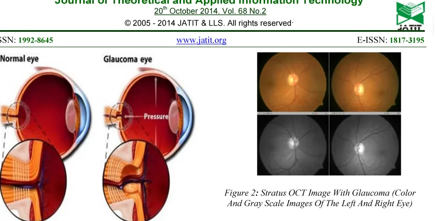
million cases of blindness (15% of the total burden of world blindness). It was reported that it has affected 60.5 million people in 2011, increasing to 79.6 by 2020 [1]. The ailment is physiologically described as the degeneration of optic nerve cells and is characterized by changes in the optic nerve head and visual field. Although Glaucomatous damage is irreversible, early detection and subsequent medical intervention by ophthalmologists is effective in slowing the progression of the disease. The medical diagram of normal eye and glaucoma affected eye with optic nerve damage due to intraocular pressure is shown in Figure 1.
The early stages of glaucoma will damage the optic nerve without incurring any symptom. The patients are not aware of the disease until the advanced stage of disease occurs which makes total blindness.
ISSN: www.jatit.org E-ISSN:
Figure 1: Medical Image Of Normal And Affected Eye
Clinically, the diagnosis of Glaucoma can be done through measurement of CDR, defined as the ratio of the vertical height of the optic cup to the vertical height of the optic disc. An increment in the cupping of Optic Nerve Head (ONH) corresponds to the increased ganglion cell death and hence CDR can be used to measure the probability of developing the disease. A CDR value that is greater than 0.65 indicates the high glaucoma risk [2]. The ONH assessment is manually performed by a trained specialist or using specialized and expensive equipment such as the Stratus OCT system.
OCT is an imaging technique capable of performing high-resolution, cross-sectional imaging. OCT enables real-time visualization of tissue microstructure. Stratus OCT Review Software brings a new level of connectivity and this new software enables users to import, view, analyze and manage Stratus OCT data at remote locations such as a laptop or personal computer. Therefore clinical OCT measurements are collected from the eye hospital for comparative analysis. Figure 2 shows the stratus OCT image of a patient with glaucoma. Both color and gray scale image of the left and right eye are shown.
Figure 2: Stratus OCT Image With Glaucoma (Color And Gray Scale Images Of The Left And Right Eye)
Thus, this imaging technique provides a cross-sectional view of examined tissue, highest axial resolution, multiple scanning regions and automatic definition of ONH margin. One of the earliest reported methods was based on the discriminatory analysis of color intensity [3]. Later, in [4], pixels within the retinal image were classified based on pixel features generated from stereo color retinal images. Variation level set based on pixel intensity was used to globally optimize the obtained cup contour in [5]. A convex hull based neuro-retinal optic cup Ellipse Optimization algorithm improves the accuracy of the boundary estimation [6]. Further enhancement of optic cup detection can be done from ARGALI key parameters such as rim volume, cup/disc area ratio, cup area and volume, disc area and volume [7]. In this study, an optimized solution for optic cup-to-disc ratio detection is focused and a comparative result of the proposed method is presented.
2. METHODOLOGY
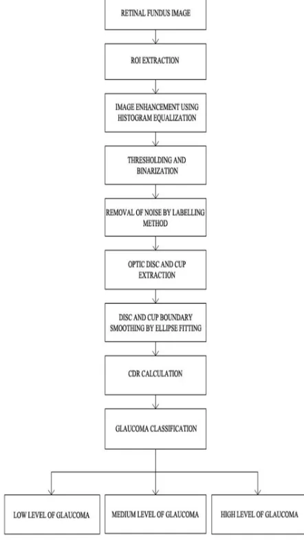
The methodology adopted for computer aided glaucoma diagnosis through CDR measurement is shown in Figure 3. It consists of different stages of preprocessing of the input image followed by disc and cup extraction to determine the cup to disc ratio. Then based on the CDR value, the glaucoma affected images are classified as (i) low level of glaucoma, (ii) medium level of glaucoma and (iii) high level of glaucoma.
2.1 ROI Determination
[image:2.595.90.301.107.302.2]ISSN: www.jatit.org E-ISSN: can be performed on the entire image, localizing the
[image:3.595.74.295.222.616.2]ROI would help to reduce the computational cost as well as improve segmentation accuracy. The component labeling method can be used to localize exact boundary. The regions labelled using the neighbourhood connecting pixels and all the connected pixels with the same input value are assigned the same identification label.
Figure 3: Simplified Work Flow Of Computer Aided Glaucoma Diagnosis Through CDR Measurement
The optic disc region is usually of a brighter pallor or higher color intensity than the surrounding retinal area. This characteristic can be exploited through automatic selection of 0.5% of the pixels in the image with the highest intensity. Next, the retinal image is subdivided into 64 regions and an approximate ROI center is selected based on the region containing the highest number of
pre-selected pixels. Then, the ROI is defined as a rectangle around the ROI centre with dimensions of twice the typical optic disc diameter and is used as the initial boundary for the optic disc segmentation.
2.2 Optic Disc Segmentation
The vertical cup to disc ratio can be calculated after segmenting the optic cup and disc regions. The optic disc extraction is straight forward and various approaches have been proposed for segmentation of the disc. The disc boundary can be detected using optimal color channel as determined by the color histogram analysis and edge analysis.
2.3 Optic Disc Smoothing
The disc boundary found from the segmentation may not represent the actual shape of the disc since the boundary can be affected by a large number of blood vessels entering the disc. Therefore, the ellipse fitting can be performed to reshape the disc boundary for better estimation.
2.4 Optic Cup Segmentation
Compared to the extraction of the optic disc, cup segmentation provides an even greater challenge, as the cup-disc boundary is usually less pronounced than that of the disc region and is further compounded the increased visibility of blood vessels across the cup-disc boundary. The cup can be extracted using image processing techniques [5].
2.5 Optic cup Smoothing
After detecting the cup boundary, the ellipse fitting can be employed to eliminate some of the cup boundary’s sudden changes in curvature. Ellipse fitting becomes especially useful when portions of the blood vessels in the neuro-retinal rim outside the cup are included with in the detected boundary. The CDR can be consequentially obtained based on the height of detected cup and disc.
2.6 Ellipse Optimization for optic disc and cup
Ellipse fitting algorithm is used to smooth the disc and cup boundary. Ellipse fitting is usually based on least square fitting algorithm which assumes that the best-fit curve of a given type is the curve that has the minimal sum of the deviations squared from a given data points (least square error).
ISSN: www.jatit.org E-ISSN: chosen to fit the optic cup over other popular ellipse
fitting algorithms like Bookstein Algorithm and Taubin Algorithm [8]. Instead of fitting general conics or being computationally expensive, this algorithm minimizes the algebraic distance subject to a constraint, and incorporates the ellipticity constraint into the normalization factor. It is ellipse-specific, thus the effect of noise (ocular blood vessel, hemorrhage, drusens, etc.) around the cup area can be minimized while forming the ellipse. It can also be easily solved by a generalized Eigen system.
In the Fitting algorithm, a quadratic constraint is set on the parameters to avoid trivial and unwanted solutions. The goal is to search a vector parameter which contains the ‘n’ coefficients of the standard form of a conic.
An ellipse is a special case of a general conic which can be described by an implicit second order polynomial
2 2
( , )
0
F x y
=
ax
+
bxy
+
cy
+
dx
+
ey
+
f
=
(1)
with an ellipse-specific constraint
2
4
0
b
−
ac
<
(2) Where a, b, c, d, e, f are coefficients of the ellipse and (x, y) are the co- ordinates of points lying on it. The polynomial F(x, y) is called the algebraic distance of the point (x, y) to the given conic. By introducing vectors
2 2
[ , , , , ,
]
T[x , xy, y , x, y,1]
P
=
a b c d e f
and Q
=
(3)
F(x,y) can be rewritten in the vector form as
( )
.
0
P
F Q
=
Q P
=
(4)The fitting of a general conic to a set of points (xi,yi), i = 1…N, may be approached by minimizing
the sum of squared algebraic distances of the points to the conic which is represented by the coefficient P:
(
)
22
1 1
min
(X , )
min
(Q )
N N
i i P i
i i
F
Y
F
= =
=
∑
∑
(5)
The Eqn. (5) can be solved by the standard least squares approach, but the result of such fitting is a general conic and it need not to be an ellipse.
To ensure an ellipse–specificity of the solution, the appropriate constraint given in Eqn. (2) has to be considered. Under a proper scaling, the inequality constraint in Eqn. (2) can be changed into an equality constrain as
2
4
ac
−
b
=
1
(6)
and the ellipse-specific fitting problem can be reformulated as
2
min
D
Psubject to P
TC
P
=
1
(7)
where the design matrix D of size N×n, represents the least squares minimization of Eqn.(5) and the constraint matrix C of size n×n, express the constraint of Eqn.(6). The Eqn. (7) can be solved by a quadratically constrained least squares minimization technique. By applying the Lagrange multipliers, the optimal solution P can be found from
1
T
P
=
λ
P and P
P
=
S
C
C
(8)where S is the scatter matrix of the size n×n, which is given as
T
=
S
D D
(9)
Eqn. (8) can be solved using generalized Eigen vectors. There exist up to ‘n’ real solutions, but by considering the minimization ||DP||2 subjected to the
constraint given in Eqn.(6) would yield only one solution, which corresponds by virtue of constraint, to an ellipse.
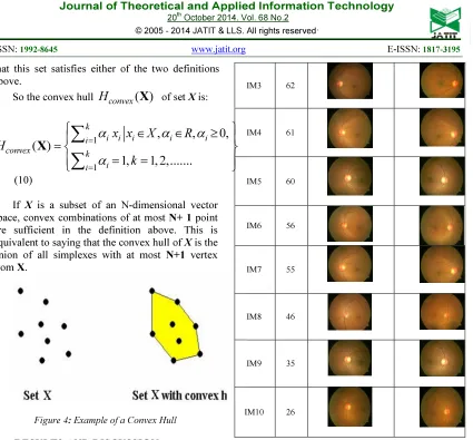
2.7 Convex hull based Ellipse Optimization A convex hull of a set of points is the smallest convex polygon that contains every one of the points [6]. It can be defined by a subset of all the points in the original set, as shown in Figure 4.The convex hull of X can also be described constructively as the set of convex combinations of finite subsets of points from X: that is, the set of points of the form ∑୬ t୨
୨ୀଵ x୨, where n is an arbitrary
ISSN: www.jatit.org E-ISSN: that this set satisfies either of the two definitions
above.
So the convex hull
H
convex( )
X
of set X is:1
1
,
,
0,
( )
1,
1, 2,...
ki i i i i i
convex k i i
x x
X
R
H
k
α
α
α
α
==
∈
∈
≥
=
=
=
∑
∑
X
(10)
If X is a subset of an N-dimensional vector space, convex combinations of at most N+ 1 point are sufficient in the definition above. This is equivalent to saying that the convex hull of X is the union of all simplexes with at most N+1 vertex from X.
Figure 4: Example of a Convex Hull
3. RESULTS AND DISCUSSION
The neuro- retinal images used for developing the system have been obtained from Vasan Eye Care Hospital, Salem. The important samples are given in Table 1. The Cup to Disc Ratio for each neuro- retinal image was provided by the ophthalmologist using stereographic viewers and images were set as ground truth against which the performance of the proposed method was evaluated.
Table 1: Retinal images for various age groups
Image Age
Oct Images
Right Eye Left Eye
IM1 74
IM2 65
IM3 62
IM4 61
IM5 60
IM6 56
IM7 55
IM8 46
IM9 35
IM10 26
[image:5.595.94.519.71.466.2]Various parameters such as rim volume, cup to disc area ratio, cup area and volume, disc area and volume have been computed to analyze the captured retinal eye image of the patients in the hospital. The CDR measurement has been done using the flow graph given in Figure.3. The sample image considered for the explanation of the estimation procedure is given in Figure.5.
ISSN: www.jatit.org E-ISSN:
(a) (b)
[image:6.595.109.286.245.379.2]Figure 6: (a) ROI before labelling (b) ROI after labelling
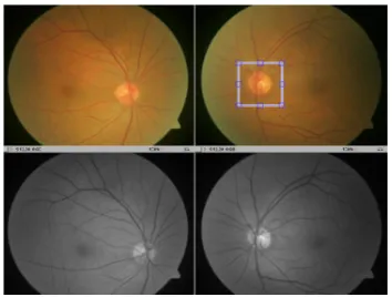
Figure 7: Retinal fundus image with the defined ROI in the outlined rectangle
The ROI has been determined and the component labeling has done to exactly extract the ROI. The extracted image is given in Figure.6. Then the ROI has been marked with rectangle for further analysis. The retinal fundus image with the defined ROI is shown in Figure 7.
(a) (b)
Figure 8: (a) Optic Disc segmented image, (b) Optic Disc smoothened image
(a) (b)
Figure 9: (A) Optic Cup Segmented Image, (B) Optic
Cup Smoothened Image
The optic disc and cup segmented from the above process are further smoothened to get exact boundary as shown in Figure 8&9 respectively.
Finally the ellipse fitted optic disc and cup is shown in Figure 10 with disc height and cup height to estimate the CDR.
Figure 10: Ellipse fitted Optic Disc and Cup
Similar processing has been done for more number of images for validating the proposed method. The experimental results have been verified and validated with standard values of the parameter for the normal eyes given in Table 2.
Table2: Normal Eye Parameters
Sl.No. Parameter Values 1 Cup to Disc Ratio 0.2 to 0.3
2 Cup to Disc Area
Ratio 0.20 ± 0.13 3 Cup Area 0.40 ± 0.33 4 Disc Area 1.93 ± 0.40
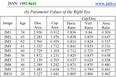
[image:6.595.307.504.390.459.2]The clinical parameters collected from the hospitals for various images both Right and Left eyes are given in Table 3. These parameters are the guiding values for comparison of estimated values derived from the proposed method.
Table 3: Clinical Data of the Patients
(a) Parameter Values of the Left Eye
Image Age Disc Area
Cup Area
Cup/Disc Horiz.
Ratio
Vert. Ratio
[image:6.595.108.528.498.690.2]ISSN: www.jatit.org E-ISSN: (b) Parameter Values of the Right Eye
Image Age Disc Area Cup Area Cup/Disc Horiz. Ratio Vert. Ratio Area Ratio IM1 74 2.956 0.912 0.836 0.84 0.309 IM2 65 2.283 1.476 0.838 0.839 0.647 IM3 62 2.760 0.929 0.810 0.824 0.337 IM4 61 3.355 1.712 0.841 0.839 0.510 IM5 60 2.729 1.303 0.712 0.725 0.477 IM6 56 1.872 1.231 0.820 0.837 0.658 IM7 55 2.139 0.765 0.637 0.624 0.358 IM8 46 2.589 1.242 0.871 0.870 0.480 IM9 35 1.483 0.654 0.751 0.749 0.441 IM10 26 3.127 1.445 0.869 0.866 0.462
[image:7.595.72.308.108.265.2]The performance of the proposed system has been validated with the clinical estimation. It can be observed that the CDR estimated using the proposed algorithm is close to the clinical estimation (Table 4).
Table 4: CDR Values of Various Images with Different Age
Image Age
CDR
Right Eye Left Eye
Clinical Method Proposed Method Clinical Method Proposed Method IM1 74 0.644 0.603 0.837 0.797
IM2 65 0.839 0.799 0.869 0.829 IM3 62 0.824 0.804 0.456 0.432
IM4 61 0.839 0.799 0.839 0.829
IM5 60 0.521 0.481 0.725 0.685
IM6 56 0.837 0.790 0.837 0.790 IM7 55 0.669 0.629 0.624 0.583
IM8 46 0.841 0.801 0.870 0.830
IM9 35 0.741 0.701 0.749 0.709
IM10 26 0.886 0.845 0.866 0.811
The risk of glaucoma is assessed based on CDR value and greater than 0.65 indicates high glaucoma. The various parameters for glaucoma assessment which are obtained by the Stratus OCT machine are collected from the VASAN EYE CARE Hospital, the first corporate chain of Eye Hospitals in India. The collected data consists of the measured parameters and the images of few patients who are affected by the glaucoma. Initially the patients are subjected to the diabetic test before the glaucoma test.
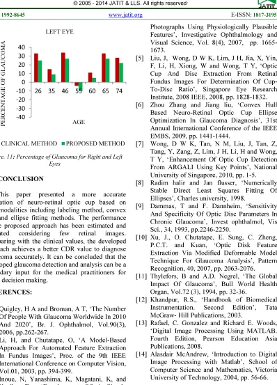
The percentage of Glaucoma has been calculated using Eqn. 11 for classification of images and shown in Table 5. From Figure.11, it has been observed that the level
of glaucoma changes from one eye to another eye, independent of age and depends only on the physical parameters of the eyes. Also it has been observed that the estimated values are very close to the clinical values and the correctness of the estimation have been verified with doctors. Finally, the images have been classified as (i) low level of glaucoma, (ii) medium level of glaucoma and (iii) high level of glaucoma compared with default value of 0.65.
CDR - CDR
% of Glaucoma = ×100 CDR
actual
base
base
(11)
Table 5: Percentage of Glaucoma
Image Age
Percentage Of Glaucoma Right Eye Left Eye Clinical Method Proposed Method Clinical Method Proposed Method IM1 74 -0.9 -7 28 22 IM2 65 29 23 33 27 IM3 62 28 24 -0.3 -0.33 IM4 61 0.3 0.2 0.3 0.3 IM5 60 -20 -26 11 5 IM6 56 0.3 0.2 0.3 0.2 IM7 55 3 -3 -4 -10 IM8 46 29 23 34 27 IM9 35 14 8 15 9 IM10 26 36 30 33 25
-40 -30 -20 -10 0 10 20 30 40
26 35 46 55 60 65 74
P E R C E N T AG E O F G L A UC O M A AGE RIGHT EYE
[image:7.595.78.525.327.598.2]ISSN: www.jatit.org E-ISSN:
Figure. 11: Percentage of Glaucoma for Right and Left
Eyes
4. CONCLUSION
This paper presented a more accurate estimation of neuro-retinal optic cup based on multimodalities including labeling method, convex hull and ellipse fitting methods. The performance of the proposed approach has been estimated and validated considering few retinal images. Comparing with the clinical values, the developed approach achieves a better CDR value to diagnose Glaucoma accurately. It can be concluded that the developed glaucoma detection and analysis can be a secondary input for the medical practitioners for better decision making.
REFERENCES:
[1] Quigley, H A and Broman, A T, ‘The Number Of People With Glaucoma Worldwide In 2010 And 2020’, Br. J. Ophthalmol, Vol.90(3), 2006, pp.262-267.
[2] Li, H, and Chutatape, O, ‘A Model-Based Approach For Automated Feature Extraction In Fundus Images’, Proc. of the 9th IEEE International Conference on Computer Vision, Vol.01, 2003, pp. 394-399.
[3] Inoue, N, Yanashima, K, Magatani, K, and Kurihara,T , ‘Development Of A Simple Diagnostic Method For The Glaucoma Using Ocular Fundus Pictures’, Conf. Proc. Of IEEE Engineering in Medicine and Biology Society, 2005, pp. 3355-3358.
[4] Abramoff, M D, Alward, W L M, Greenlee, E C, Shuba, L, Kim, C Y, Fingert, J H and Kwon, Y H, ‘Automated Segmentation Of The Optic Disc From Stereo Color
Photographs Using Physiologically Plausible Features’, Investigative Ophthalmology and Visual Science, Vol. 8(4), 2007, pp. 1665-1673.
[5] Liu, J, Wong, D W K, Lim, J H, Jia, X, Yin, F, Li, H, Xiong, W and Wong, T Y, ‘Optic Cup And Disc Extraction From Retinal Fundus Images For Determination Of Cup-To-Disc Ratio’, Singapore Eye Research Institute, 2008 IEEE, 2008, pp. 1828-1832. [6] Zhou Zhang and Jiang liu, ‘Convex Hull
Based Neuro-Retinal Optic Cup Ellipse Optimization In Glaucoma Diagnosis’, 31st Annual International Conference of the IEEE EMBS, 2009, pp. 1441-1444.
[7] Wong, D W K, Tan, N M, Liu, J, Tan, Z, Tang, Y, Zang, Z, Lim, J H, Li, H and Wong, T Y, ‘Enhancement Of Optic Cup Detection From ARGALI Using Key Points’, National University of Singapore, 2010, pp. 1-5. [8] Radim halir and Jan flusser, ‘Numerically
Stable Direct Least Squares Fitting Of Ellipses’, Charles university, 1998.
[9] Dammas, T and F. Dannheim, ‘Sensitivity And Specificity Of Optic Disc Parameters In Chronic Glaucoma’, Invest ophthalmol, Vis Sci., 34, 1993, pp.2246-2250.
[10] Xu, J., O. Chutatape, E. Sung, C. Zheng, P.C.T. and Kuan, ‘Optic Disk Feature Extraction Via Modified Deformable Model Technique For Glaucoma Analysis’, Pattern Recognition, 40, 2007, pp. 2063-2076. [11] Thylefors, B and A.D. Negrel, ‘The Global
Impact Of Glaucoma’, Bull World Health Organ, Vol.72 (3), 1994, pp. 32-36.
[12] Khandpur, R.S., ‘Handbook of Biomedical Instrumentation. Second Edition’, Tata McGraw- Hill Publications, 2003.
[13] Rafael, C. Gonzalez and Richard E. Woods, ‘Digital Image Processing Using MATLAB. Fourth Edition, Pearson Education Asia Publications, 2008.
[14] Alasdair McAndrew, ‘Introduction to Digital Image Processing with Matlab’, School of Computer Science and Mathematics, Victoria University of Technology, 2004, pp. 56-66. -40
-30 -20 -10 0 10 20 30 40
26 35 46 55 60 65 74
P
E
R
C
E
N
T
AG
E
OF
GL
A
UC
O
M
A
AGE LEFT EYE