HYBRID OPTIMIZATION FOR GRID SCHEDULING USING GENETIC ALGORITHM WITH LOCAL SEARCH

(1)

ISSN: 1992-8645 www.jatit.org E-ISSN: 1817-3195

INTELLIGENT

IRRIGATION

WATER

REQUIREMENT

SYSTEM

BASED

ON

ARTIFICIAL

NEURAL

NETWORKS

AND

PROFIT

OPTIMIZATION

FOR

PLANTING

TIME

DECISION

MAKING

OF

CROPS

IN

LOMBOK

ISLAND

MOHAMMAD ISA IRAWAN1 , SYAHARUDDIN2,

DARYONO BUDI UTOMO2, ALVIDA MUSTIKA RUKMI4

Institut Teknologi Sepuluh Nopember, Faculty of Mathematics and Natural Sciences

Department of Mathematics, Surabaya

E-mail: [email protected] ,2[email protected] 3_{[email protected]}_,4_{[email protected]}

ABSTRACT

Cropping pattern is a scheduling for farming time on a certain land in a definite period (e.g. 1 year), including unfilled area. In arranging crop planting patterns, hydrological (rainfall), climatological (temperature, humidity, wind speed, and sunshine), crop (crop coefficient value, productivity and price) and land area data are required. Therefore, a method that can be applied to predict the hydro climatological data is needed.

The appropriate method for such prediction is Back Propagation Neural Network (BPNN). Prediction result of BPNN will be used to determine minimum crop water requirements, and it will be associated with planting time (age) of each crop for making cropping pattern. The design of most favorable cropping pattern will obtain the maximum profit and reduce fail harvest problem, which in turns it can contribute to national food resilience.

Based on the simulation result, it was known that the BPNN with two hidden layers is able to predict hydro climatological data such as of rainfall, temperature, humidity, wind speed, and sunshine data with an average accuracy rate of 95.72% - 96.61%. Meanwhile, validation of predictions obtained an average percentage error of 1.12% with an accuracy of 99.76%. The results of the optimization of the cropping pattern in Lombok in March 2013-February 2014 revealed an accurateness of profit in each district/city in East Lombok, Central Lombok, West Lombok, North Lombok, and Mataram increased 2.02%, 16.88%, 20, 23%, 21.89%, and 5.58%, respectively. Over all, the increasing average was found to be 13.3% from the previous year.

Keywords: Crop, Rainfall, Back Propagation Neural Network (BPNN), Optimization.

1. INTRODUCTION

Cropping pattern is defined as making time management for planting on a certain area in a definite period (as an example, 1 year period of time) including filled area [9]. The data required in cropping patterns planning are hydrological (rainfall), climatological (temperature, humidity, wind speed, and sunshine), raw crop (as well as crop coefficient, productivity and selling price), and land area data. The data are used to calculate water requirement and alternative planting time of crop [2]. A cropping pattern planning is needed to obtain

the maximum product, quality and grade of farming. Besides that, the cropping pattern planning is also aimed to determine the amount of fertilizer and seeds which should be distributed to farmer groups in certain areas during the planting season each year.

(2)

production quantities (ton). It is due to changes and shifting seasons [5]. One of the main indicators of shifting seasons is the irregular rainfall pattern. This phenomena makes the farmers in NTB, especially Lombok, find some difficulties in determining cropping patterns of crop or horticulture.

For that reason, a study about crop planting patterns is then required, particularly for generating a method in anticipating climate changes in order to keep the products and sustainable food even better. Such method is also reliable to predict the hydro climatological data in the future. One of the reliable methods to predict any time series in the future is Back Propagation Neural Network (BPNN) [13].

BPNN is a well-known popular neural network algorithm for which it can solve a specific problem like pattern recognition or classification through the process of learning [4]. It poses excellent and high accuracy to predict time series data [6]. A BPNN with two hidden layers screen is able to provide better and faster prediction results compared to a BPNN with only one hidden layer [12]. Then Nastos [7], has conducted a study to build a prediction model to predict the intensity of rainfall data (mm/day) in Athens, Greece. The results showed that the BPNN is trustworthy in making predictions of future rainfall data, it was claimed as a satisfactory method by evaluators of the network using the Mean Absolute Error (MAE), Mean Bias Error (MBE), Root Mean Square Error (RMSE), coefficient of Determination (R2), and the Index of Agreement (IA).

The prediction results which were obtained by means of BPNN were used to determine the effective rainfall, evapotranspiration, and minimum water requirements for crop. Afterward, optimization of production profit was to gain maximum profit with low cost. The optimization results with highest profit (income) and minimum water requirements will be recommended as cropping patterns to be adopted by farmers for the next planting season. This planting pattern is expected as a consideration in making decision of good crop, appropriate, and optimal plants. Generally, it can be proposed as reference material in the distribution of fertilizers and crop seeds to farmer’s groups in each region in Lombok (NTB).

2. RESEARCH METHODS

The data consists of (1) hydrological data (17 posts of rainfall), (2) climatological data (humidity, temperature, sunshine, and wind speed)

comprising 4 posts of climate in Lombok Island area during 30 years (983 to 2012) of the Water Resources Information Center (WRIC) in NTB, and (3) data on agriculture (crop, income, profits, and farming production costs).

The stages in this research we divide into 3 main sections namely,

a. Predicting the hydrological data and climatological data, this step aims to determine the value from evaporation, evapotranspiration, effective rainfall, rainfall mainstay, and the need for water treatment

b. Optimizing the profits of farm produce, this step aims to determine the amount of benefits based on income and cost of production using crop land constraint functions.

c. Calculating the crop water requirements minimum, this step aims to determine when planting food based evapotranspiration, effective rainfall, and decision making.

The flow chart of research procedure is presented in Figure 1.

2.1 Crop

Crop is defined as any kind of plants that can produce carbohydrates and protein. The crop were divided into three (3) major groups, namely rice, pulse and nut [9]. Food crop in general are seasonal crop such as rice, corn, soybean, green bean, peanut, cassava, and sweet potato, but there are some crop that are perennial crop such as breadfruit and sago.

2.2 Rainfall

The nature of rain is divided into three criteria: (1) Above Normal (AN) if the value of the ratio of rainfall during 1 month on average (30 years)> 115%, (2) Normal (N) if the value of the comparison amount of rainfall for 1 month on average (30 years) between 85-115%, and (3) Under Normal (UN) if the value of the ratio of rainfall during 1 month on average (30 years) <85% [10].

(3)

% 100 × =

WM DM

Q (1)

[image:3.612.98.518.76.573.2]

Table 1. Classification of Climate Types Based on Monthly Rainfall [10].

Climate

Type Values Q (%)

Area Category

A < 14.3 Very wet

B 14.3 – 33.3 Wet

C 33.3 – 60.0 Dampy

D 60.0 – 100.0 Medium

E 100.0 – 167.0 A little dry

F 167.0 – 300.0 Dry

G 300.0 – 700.0 Very dry

H > 700.0 Exceptional

dry

Figure 1: Flow Chart of Research Procedure

2.3 Crop Water Requirement

Calculation of irrigation the water is obtained from the location rate of the area the water (P), evaporation (Ea, Ep and Eo), evapotranspiration (Eto and Etc), the land preparation the water requirement (300 and IR-200), the effective rainfall (Reff), the water turnover (WLR), and irrigation efficiency [1]. Where all variables calculation using the data obtained from

the results predicted of rainfall, temperature, humidity, wind speed, and sunshine.

2.3.1 Evaporation

In determining the magnitude of evaporation used by Penman method (1948) in [2], explicitely,

(

e e

)(

u

)

E_a =0.35 _s − _a 0.5+0.54 (2) No

Ye s

Validation Start

Average Rainfall

Rainfall Mainstay

Effective Rainfall

Evaporation

Evapotranspiration Water Processing of Land

Water Requirement

Irrigation

Finish

Wind Speed Data

Humidity Data

Sunshine Data

Temperature Data

Prerprocessing

Prediction

Post-processing

Data Collection

(Field, Department of Agriculture in

Algorithm BPNN

Architecture

BPNN

Design of Planting Pattern

Crops Data

Climatology Data

Hydrology Data

The First Planting Pattern

Optimization of Profits with QM for Windows

Optimal Cropping

Pattern

Rainfall

Data

(4)

where es value is depent on the temperature of an area. The ea is obtained by multiplying the

relative humidity (h) with es

(

e

a

=

h

×

e

s

)

. Then

u value is the wind speed (m/s).

2.3.2 Evapotranspiration

The magnitude of evapotranspiration is affected by the radiation, the slope of the saturated vapor pressure curve, and evaporation.

1) Radiation (R, Ra, Rb, Rc, R1)

( )

(

× = − 10 4 .

117 9 Ta 4

Rb

( )

(

)

      + − × = − 100 8 . 0 20 . 0 77 . 0 47 . 0 10 4 .

117 9Ta4 e m

R_b _a (3)

where Ta=273.3+T Rc is then













+

=

100 m

b

a

R

_c _a (4)

where a =0.28,b=0.48, R_a =949

Rc values in equation 4 is used to determine the value of R1, thus,

( )

r R

R₁= _c1− (5)

where r = 0,25.

Then the value of Rb in equation 3 and R1 in equation 5 is used to determine the value of R, or,

b

R R

R= ₁− ₍₆₎

2) The slope of the curve Saturated Vapor Pressure

(

)

2

3 . 237 27 . 17 3 . 273 6108 . 0 4098 +         = ∆       + T e T T (7)

3) Evapotranspiration (Ep, Eto)

Using equation 2, 6, and 7 we get value of

Ep,

1 ×

(10)

Furthermore, using equation 10, we obtain the magnitude of evapotranspiration formula of Penman (1948) in Shen et al [11], as given below,

o c

c

K

Et

=

.

(11)

2.3.3 Water Requirement Processing

The magnitude of water requirements at the time of land preparation can be calculated using the methods developed by Van de Goordan Zilstra (1968) in Allen et al [2] IR values determined using equation 10, thus obtained,

1 − = _k k

e Me

IR (12)

where k=MT/S, M =Eo +P, e=2.7182, S

= 250 or S = 300 and P = 3.

2.3.4 Effective Rainfall

Effective rainfall is the rainfall that falls on an area of agriculture in which can only partially be used or absorbed by plants to meet requirement as long of growth. The magnitude of effective rainfall is determined by 70% of the of mainstay rainfall (R80) for rice and (R50) for a non-rice food crops (palawija). The steps in determining effective rainfall following.

1) Determining Average Rainfall

n R R R R

R= 1+ 2+ 3+...+ n

(13) 2) Determining Mainstay Rainfall

a) For Rice : ₁ 5

80= + N

R (14)

b) For Palawija: ₁

2

50= + N

R (15)

3) Determining Effective Rainfall (Reff) a) For Rice :

15 7 . 0 R80

R_eff = × (16)

b) For Palawija:

15 7 . 0 R50

Reff = × (17)

Based on equations 11 and 17, then get the equation for determining the water requirement for irrigation as given below,

1) Water Requirement for Rice

WLR R

P Et

NFR= c+ − eff + (18)

2) Water Requirement for Palawija

eff c P R

Et

NFR = + − (19)

(5)

with the efficiency of crop water requirements. Therefore, by using equation 18 (for rice) the equation below is then acquired,

64 . 8 65 . 0 64 . 8 × + − + = ×

= Et P R WLR

E NFR

DR c eff (20)

2.4 FORCASTING WITH BACK

PROPAGATION NEURAL NETWORK 2.4.1 Types Of Forecasting Using Bpnn

The time series data forecasting with ANN consists of two types, namely:

Short term prediction:

(

₋₁, ₋₂, ₋₃,...

)

= k k k

k NN y y y

y (21)

Long term prediction:

(

, 1, 2, 3,...

)

1 − − −

+ = k k k k

k NN y y y y

y (22)

In this research,

y

_k is the prediction result in 2013 using data for 1983 to 2012, while

1 +

k

y

is the prediction results in 2014 using data for 1983 to 2012 and prediction result in 2013.

2.4.2 Evaluation Of Prediction Result

For testing the validity of forecast or evaluation of prediction results these used forecast accuracy. Wilmott (1982) in Nastos [7], gave some of the criteria to evaluate that prediction results, i.e. Mean Absolute Error (MAE), Mean Bias Error (MBE), Mean Square Error (MSE), Root Mean Square Error (RMSE), coefficient of Determination (R2), and the Index of Agreement (IA).

1) Mean Absolute Error (MAE)

n O P MAE n i i i

∑

= −

= 1 ₍₂₃₎

2) Mean Bias Error (MBE)

(

)

n O P MBE n i i i

∑

= − = 1 (24)

3) Mean Square Error (MSE)

(

)

n O P MSE n i i i

∑

= − = 1 2 (25)

4) Root Mean Square Error (RMSE)

(

)

2

1 1 2             − =

∑

= n O P RMSE n i i i (26) 5) Coefficient of Determination (R2)

(

)

(

)

∑

= =

−

=

_n i ave i i n i i i

O

P

O

R

1 2 1 2 2

1

(27)

6) Index of Agreement (IA)

(

)

(

)

∑

= = − + − − − = _n i ave i i ave i i n i i i O O O P P O IA 1 2 1 2 1 (28)

2.5 Optimization Of Crop

Optimization of the planting pattern is designed in order to obtain the maximum profit. A frequently applied method in farming analysis is Linear Programming (LP) regarding to the use or the efficient allocation of limited resources to achieve desired goals [8]. Jasbir [3] introduced the following definition of a standard LP,

a. Objective Function

∑

= = + + + + = n j j j n n

j cx cx cx cx cx

Z 1 3 3 2 2 1 1 ... (29)

b. Function Constraints (Limiting Factor) Maximize:

∑

= ≤        ≤ + + + + ≤ + + + + ≤ + + + + n j i j ij m n mn m m m n n n n b x a b x a x a x a x a b x a x a x a x a b x a x a x a x a 1 3 3 2 2 1 1 2 2 3 23 2 22 1 21 1 1 3 13 2 12 1 11 ... ... ... M Minimize:

∑

= ≥        ≥ + + + + ≥ + + + + ≥ + + + + n j i j ij m n mn m m m n n n n b x a b x a x a x a x a b x a x a x a x a b x a x a x a x a 1 3 3 2 2 1 1 2 2 3 23 2 22 1 21 1 1 3 13 2 12 1 11 ... ... ... M

c. Conditions (Assumption)

0 ,

,

0 ,

,

3 2 1 3 2 1

≥

m n

b

x

From the above definition, we can identify indicators of crop planting pattern optimization (farming) as follows,

a. Determinant Variable (related)

The determinant variables in the optimization is divided into two variables, namely:

The dependent variable, containing income (ZP), production costs (ZB), and profit (ZL).

(6)

cassava, the production quantity (J1, J2, ..., J7), price sales by kg (H1, H2, ..., H7), production costs (B1, B2, ..., B7), which consists of the cost of seeds, irrigation, fertilizers, plows (tractor engine), pesticides (insecticides and fungicides), labor (planting, care of, harvest, and so on), the area of each plant (L1, L2, ..., L7), and the maximum area (L).

b. Objective Function (maximize of profit)

Income (ZP). The income (ZP) is obtained from the multiplication of the quantity of production, selling price of crop, and the land area of each crop type, in order to acquire,

7 7 7 2 2 2 1 1

1 ) ( ) ... ( )

(J H X J H X J H X

Z_P= × + × + + ×

(30)

Production Costs (ZB). The production costs (ZB) is obtained from the multiplication of the production costs of crop and land area of each type of crop, in order to attain,

L

Z

=

−

(32)

Hence, the objective function can be expressed as follows

[

]

(

)

[

]

∑

= − × = × + + − × = 7 1 7 7 7 1 1 1

1 ) ... ( )

( i i i i i L X B H J X H J X B H J

Z ₍₃₃₎

c. Function Constraints

By using land area planted for each crop (LnTn) and the maximum area (L), the constraint functions can be obtained below,

0 ,... , , 0 ,... , , ... ... ... 7 . 3 3 . 1 2 . 1 1 . 1 7 3 2 1 7 7 . 3 3 3 . 3 2 2 . 3 1 1 . 3 7 7 . 2 3 3 . 2 2 2 . 2 1 1 . 2 7 7 . 1 3 3 . 1 2 2 . 1 1 1 . 1 ≥ ≥ ≤ + + + + ≤ + + + + ≤ + + + + L L L L X X X X L X L X L X L X L L X L X L X L X L L X L X L X L X L M

while the Linear Programming (Optimization) performed using QM for Windows.

3. RESULTS AND DISCUSSION

3.1 Implementation And Validation Architecture Of Bpnn

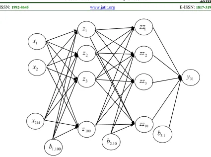
The input in this research is half of the monthly (15 days) for 30 years. Each of the data contained 24 data, so that the total data is 720 data (24 x 30 years). The Neural Network Back Propagation (BPNN) architecture design was executed to determine the best architecture with certain parameter settings through training and testing data which had been divided before. The architectural parameters are given as following:

1. Neuron Numbers : a. Input layer : 744

b. Hidden 1 layer : 100 c. Hidden 2 layer : 10 d. Output layer : 1 2. Activation Function: Sigmoid Biner 3. Training Algorithm: trainrp

4. Setting Parameter:

a. Max. Epoch : 10000

b. Error (Goal) : 0.0001 c. Learning Rate (LR) : 0.07

d. Momentum : 0.9

e. Decreased ratio of LR : 0.7 f. Increased ratio of LR : 1.05

(7)

Figure 2: Back Propagation Neural Networks with Two Hidden Layers for Prediction

The designed architecture can be treated to calculate the percentage of accuracy evaluated (P) by comparing the same pattern (Q) for all patterns (R).

% 100

× =

R Q

P (34)

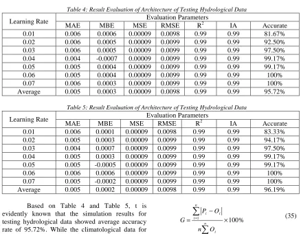
[image:7.612.92.517.67.383.2]

The simulation results using equations 23, 24, 25, 26, 27, 28, and 34 for training hydrological data and climatological data are presented in Table 2 and Table 3, then for testing hydrological data and climatological data are presented in Table 4 and Table 5 then that’s shown on Table 4 and Table 5,

Table 2: Result Evaluation of Architecture of Training Hydrological Data

Learning Rate Evaluation Parameters

MAE MBE MSE RMSE R2 IA Accuration

0.01 0.005 -0.00005 0.00009 0.0098 0.99 0.99 84.96%

0.02 0.005 0.0002 0.00009 0.0099 0.99 0.99 95.11%

0.03 0.006 0.0004 0.00009 0.0099 0.99 0.99 98.37%

0.04 0.004 0.0002 0.00009 0.0099 0.99 0.99 99.28%

0.05 0.005 -0.0002 0.00009 0.0099 0.99 0.99 99.09%

0.06 0.006 0.0003 0.00009 0.0099 0.99 0.99 99.46%

0.07 0.005 0.0002 0.00009 0.0099 0.99 0.99 100%

(8)

Table 3: Result Evaluation of Architecture of Training Climatological Data

MAE MBE MSE RMSE R2 IA Accurate

0.01 0.005 0.00004 0.00009 0.0098 0.99 0.99 85.14%

0.02 0.004 0.00006 0.00009 0.0099 0.99 0.99 94.02%

0.03 0.004 -0.0001 0.00009 0.0099 0.99 0.99 96.74%

0.04 0.004 0.00003 0.00009 0.0099 0.99 0.99 98.91%

0.05 0.004 0.0001 0.00009 0.0099 0.99 0.99 99.64%

0.06 0.005 -0.00003 0.00009 0.0099 0.99 0.99 99.82%

0.07 0.006 0.0001 0.00009 0.0099 0.99 0.99 100%

Average 0.005 0.00003 0.00009 0.0098 0.99 0.99 96.32%

[image:8.612.87.525.284.624.2]

Based on Table 2 and Table 3, it is clearly known that the simulation results for the training hydrological data showed average accuracy rate of 96.61%. While the climatological data for training revealed average accuracy rate of 96.32%.

Table 4: Result Evaluation of Architecture of Testing Hydrological Data

0.01 0.006 0.0006 0.00009 0.0098 0.99 0.99 81.67%

0.02 0.006 0.0005 0.00009 0.0099 0.99 0.99 92.50%

0.03 0.006 0.0005 0.00009 0.0099 0.99 0.99 97.50%

0.04 0.004 -0.0007 0.00009 0.0099 0.99 0.99 99.17%

0.05 0.005 0.0004 0.00009 0.0099 0.99 0.99 99.17%

0.06 0.005 0.0004 0.00009 0.0099 0.99 0.99 100%

0.07 0.006 0.0003 0.00009 0.0099 0.99 0.99 100%

Average 0.005 0.0003 0.00009 0.0098 0.99 0.99 95.72%

Table 5: Result Evaluation of Architecture of Testing Hydrological Data

0.01 0.006 0.0001 0.00009 0.0098 0.99 0.99 83.33%

0.02 0.005 0.0003 0.00009 0.0099 0.99 0.99 94.17%

0.03 0.004 0.0007 0.00009 0.0099 0.99 0.99 97.50%

0.04 0.005 0.0003 0.00009 0.0099 0.99 0.99 99.17%

0.05 0.005 -0.0005 0.00009 0.0099 0.99 0.99 99.17%

0.06 0.006 0.0006 0.00009 0.0099 0.99 0.99 100%

0.07 0.005 -0.0002 0.00009 0.0099 0.99 0.99 100%

Average 0.005 0.0002 0.00009 0.0098 0.99 0.99 96.19%

Based on Table 4 and Table 5, t is evidently known that the simulation results for testing hydrological data showed average accuracy rate of 95.72%. While the climatological data for testing indicated average accuracy rate of 96.19%.

Above all, the data in 2012 can be well predicted by using the 1983 to 2011 data. The prediction results was compared with the actual data in 2012 to know the percentage of error of prediction results, which was calculated by the equation below [7].

% 100

1

1 _×

− =

∑

= =

n

i i n

i

i i

O n

O P

G (35)

where

P

_i result prediction data in 2012 and

O

_i actual data in 2012.

(9)

Table 6: Error Value of Prediction Architecture of Hydroclimatological data

Data Type Acuration Error

Percentage

Rainfall 99.73 % 2.78 %

Temperature 99.63 % 0.20 %

Humidity 99.78 % 0.45 %

Wind Speed 99.90 % 1.45 %

Sunshine 99.77 % 0.74 %

Average 99.76 % 1.12 %

According to Table 6, it is known that the average error of the predictions using the

architecture that has been designed is 1.2%. The architecture which used to predict is fairly good with average accuracy rate of 99.76%.

3.2 Prediction Result Of Hydrological Data

[image:9.612.92.518.265.444.2]

From the results of the prediction (using equation 13), it is known that the average rainfall in Lombok Island in 2013 is 65.95 mm. While in 2014, the average of rainfall is 63.47 mm in Lombok, as in Figure 3 and Figure 4.

[image:9.612.94.520.472.635.2]

Figure 3: Prediction Result of Rainfall of ½ Monthly of Lombok in 2013

Figure 4: Prediction Result of Rainfall of ½ Monthly of Lombok in 2014

3.3 Prediction Result Of Climatologycal Data

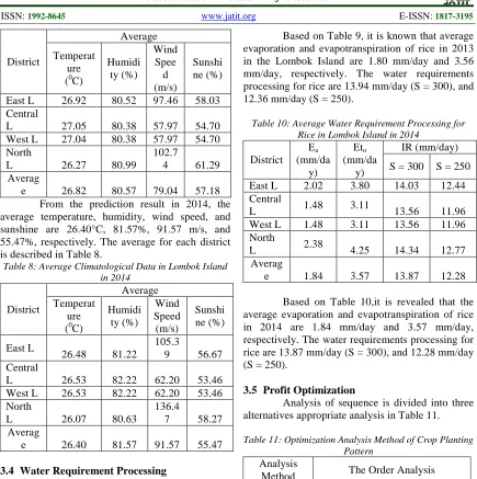
From the prediction results (using equation 13), it is revealed that during 2013, the average temperature, humidity, wind speed, and sunshine,

are 26.82°C, 80.57%, 79.04 m/s, and 57.18%, respectively. The average for each district is described in Table 7.

Table 7: Average Climatological Data in Lombok Island in 2013

0 20 40 60 80 100 120 140 160

-1 4 9 14 19 24

rai

n

fal

l

1/2 Monthly

0 20 40 60 80 100 120 140 160

-1 4 9 14 19 24

rai

n

fal

l

(10)

District

Average

Temperat ure (0C)

Humidi ty (%)

Wind Spee

d (m/s)

Sunshi ne (%)

East L 26.92 80.52 97.46 58.03 Central

L 27.05 80.38 57.97 54.70

West L 27.04 80.38 57.97 54.70 North

L 26.27 80.99

102.7

4 61.29

Averag

e 26.82 80.57 79.04 57.18

[image:10.612.90.525.67.504.2]

From the prediction result in 2014, the average temperature, humidity, wind speed, and sunshine are 26.40°C, 81.57%, 91.57 m/s, and 55.47%, respectively. The average for each district is described in Table 8.

Table 8: Average Climatological Data in Lombok Island in 2014

District

Average Temperat

ure (0C)

Humidi ty (%)

Wind Speed (m/s)

Sunshi ne (%)

East L

26.48 81.22

105.3

9 56.67

Central

L 26.53 82.22 62.20 53.46

West L 26.53 82.22 62.20 53.46 North

L 26.07 80.63

136.4

7 58.27

Averag

e 26.40 81.57 91.57 55.47

3.4 Water Requirement Processing

From the analysis result (using equations 2, 3, 4, 5, 6, 7, 8, 9, 10, 11, and 12) about the temperature data, humidity data, sunshine data, and wind speed data obtained average water requirements processing (early planting) for rice plants as described in Table 9 and Table 10.

Table 9: Average Water Requirement Processing for Rice in Lombok in 2013

District Ea (mm/da

y)

Eto (mm/da

y)

IR (mm/day)

S = 300 S = 250

East L 2.03 3.84 14.13 12.56

Central L

1.58 3.27

13.74 12.15

West L 1.58 3.27 13.74 12.15

North L

2.02 3.84

14.14 12.57 Averag

e 1.80 3.56 13.94 12.36

Based on Table 9, it is known that average evaporation and evapotranspiration of rice in 2013 in the Lombok Island are 1.80 mm/day and 3.56 mm/day, respectively. The water requirements processing for rice are 13.94 mm/day (S = 300), and 12.36 mm/day (S = 250).

Table 10: Average Water Requirement Processing for Rice in Lombok Island in 2014

District Ea (mm/da

y)

Eto (mm/da

y)

IR (mm/day)

S = 300 S = 250

East L 2.02 3.80 14.03 12.44

Central

L 1.48 3.11 13.56 11.96

West L 1.48 3.11 13.56 11.96

North

L 2.38 4.25 14.34 12.77

Averag

e 1.84 3.57 13.87 12.28

Based on Table 10,it is revealed that the average evaporation and evapotranspiration of rice in 2014 are 1.84 mm/day and 3.57 mm/day, respectively. The water requirements processing for rice are 13.87 mm/day (S = 300), and 12.28 mm/day (S = 250).

3.5 Profit Optimization

Analysis of sequence is divided into three alternatives appropriate analysis in Table 11.

Table 11: Optimization Analysis Method of Crop Planting Pattern

Analysis

Method The Order Analysis

Analysis I Planting Season I

Planting Season II

Planting Season

III Analysis II Planting

Season II

Planting Season

III

Planting Season

I Analysis III Planting

Season III

Planting Season I

Planting Season

II

The objective function and constraint function in the profit optimization:

Objective Function: Maximize (Profit):

(

)

[

]

7 6

5 4

3 2

1 7

1

54101000 35306000

13373500 21639000

8411595 8551000

34837580

X X

X X B H J Z

i

i i i i L

+ +

=

− ×

=

∑

[image:10.612.92.301.311.482.2]

(11)

Constraint function (East Lombok in 2012): Analysis I: 0 , , , , , , 5466 4 5466 4 19646 83 1 156 1 792 7 0515 1 19646 818 1098 1653 7792 8285 7 6 5 4 3 2 1 1 6 5 2 1 7 4 3 2 1 ≥ ≤ ≤ + + + ≤ + + + + X X X X X X X X X X X X X X X X X Analysis II: 0 , , , , , , 19646 19646 19646 83 1 156 1 18307 45466 818 1098 1653 5584 1 26313 7 6 5 4 3 2 1 1 6 5 1 7 4 3 2 1 ≥ ≤ ≤ + + ≤ + + + + X X X X X X X X X X X X X X X X Analysis III: 0 , , , , , , 19646 19646 45466 83 1 156 1 44127 19646 818 1098 1653 5584 1 493 7 6 5 4 3 2 1 1 6 5 1 7 4 3 2 1 ≥ ≤ ≤ + + ≤ + + + + X X X X X X X X X X X X X X X X

[image:11.612.86.526.252.338.2]

With the same method obtained constraint functions for Central Lombok, West Lombok, North Lombok and Mataram. The optimization results is presented in Table 12.

Table 12: Recommendations of Analysis Method of Crop Planting Pattern in 2012

District/city Profit (IDR) Analysis

Recomendation

I II III

East Lombok 5.08 x 109 6.79 x 109 1.00 x 1010 Analysis III

Central Lombok 7.58 x 109 8.18 x 109 9.11 x 109 Analysis III

West Lombok 4.39 x 109 4.53 x 109 4.64 x 109 Analysis III

Mataram 6.53 x 109 6.72 x 109 6.60 x 109 Analysis II

North Lombok 3.55 x 109 3.58 x 109 3.79 x 109 Analysis III

Based on Table 12, it can be seen the comparison and the percentage of profit before and after optimization is presented in Table 13.

Table 13: Comparison and Percentage of Profit before and after Optimization in 2012

District/city After Optimization (IDR) Before Optimization (IDR) Difference (IDR) Percentage of Profit (%)

East Lombok 2.55 x 1012 2.525 x 1012 2.79 x 1010 1.10

Central Lombok 4.24 x 1012 3.631 x 1012 6.10 x 1011 16.80

West Lombok 1.43 x 1012 1.224 x 1012 2.07 x 1011 16.93

Mataram 1.98 x 1011 1.829 x 1011 1.53 x 1010 8.39

North Lombok 5.95 x 1011 5.081 x 1011 8.70 x 1010 17.13

Average 1.80 x 1012 1.61 x 1012 1.89 x 1011 12.1

Based on Table 13, it is shown that there exist increasing in the percentage profit from 2011 to 2012, indicating the optimizing the results of farming with cropping patterns. Explicitly, the increasing in the percentage profit in East Lombok, Central Lombok, West Lombok, North Lombok, and Mataram increased 1.10%, 16.80%, 16,93%, 17.13%, and 8.39%, respectively. Hence, the average percentage increased 12.10% from the previous year.

Based on the above results, the optimization profit in 2013 can be calculated by means the following steps.

1. The objective function is the same as the objective function in 2012 (equation 36). 2. Constraint Function (East Lombok in 2013)

[image:11.612.88.521.391.501.2]

(12)

With the same method, constraint functions can be obtained for Central Lombok, West Lombok,

North Lombok and Mataram. The optimization results is presented in Table 14.

Table 14: Recommendations of Analysis Method of Crop Planting Pattern in 2013

District/city Profit (IDR) Analysis

Recommendation

I II III

East Lombok 4.03 x 109 5.04 x 109 6.68 x 109 Analysis III

Central Lombok 7.55 x 109 8.16 x 109 9.11 x 109 Analysis III

West Lombok 4.55 x 109 4.63 x 109 4.69 x 109 Analysis III

Mataram 5.87 x 109 6.48 x 109 6.07 x 109 Analysis II

North Lombok 3.71 x 109 3.72 x 109 3.80 x 109 Analysis III

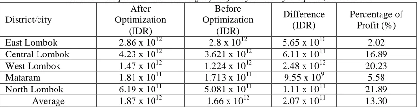
[image:12.612.90.521.277.388.2]

Based on Table 14, the comparison and the percentage of profit before and after optimization can be then calculated as it is presented in Table 15.

Table 15: Comparison and Percentage of Profit Before and After Optimization in 2012

District/city

After Optimization

(IDR)

Before Optimization

(IDR)

Difference (IDR)

Percentage of Profit (%)

East Lombok 2.86 x 1012 2.8 x 1012 5.65 x 1010 2.02

Central Lombok 4.23 x 1012 3.621 x 1012 6.11 x 1011 16.89

West Lombok 1.47 x 1012 1.224 x 1012 2.48 x 1012 20.23

Mataram 1.81 x 1011 1.713 x 1011 9.55 x 109 5.58

North Lombok 6.19 x 1011 5.081 x 1011 1.11 x 1011 21.89

Average 1.87 x 1012 1.66 x 1012 2.07 x 1011 13.30

Based on Table 15, it is known that the increment of the percentage profit from 2012 to 2013 was also found. The increasing of the percentage profit in East Lombok, Central Lombok, West Lombok, North Lombok, and Mataram are 2.02%, 16.89%, 20, 23%, 21.89%, and 5.58%. The average percentage increase 13.30% from the previous year.

3.6 Planning Cropping Patterns

From the analysis (using equations 18, 19, 20) by computing crop water requirements in 24 alternative planting time, then we can obtain an

[image:12.612.93.519.580.668.2]

alternative recommendation to planting time with minimum water requirements in each district/city, as shown in Table 16,

Table 16: Results Optimization of Crop Water Requirement

District Recommendation NFR (mm/day) DR (mm/day)

Total Average

East Lombok Alternative of 23 177.22 7.38 31.56

Central Lombok Alternative of 10 153.71 6.40 27.37

West Lombok Alternative of 23 178.01 7.42 31.69

Mataram Alternative of 12 180.06 7.50 32.06

North Lombok Alternative of 7 164.74 6.86 29.33

(13)

[image:13.612.88.526.59.709.2]

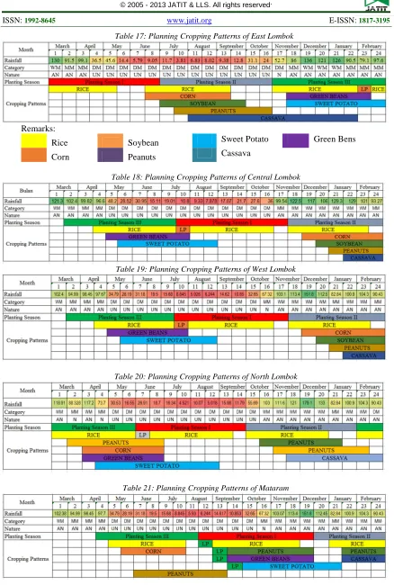
Table 17: Planning Cropping Patterns of East Lombok

Remarks:

Rice Soybean Sweet Potato Green Bens

Corn Peanuts Cassava

Table 18: Planning Cropping Patterns of Central Lombok

Table 19: Planning Cropping Patterns of West Lombok

Table 20: Planning Cropping Patterns of North Lombok

Table 21: Planning Cropping Patterns of Mataram

(14)

From the Table 17, the cropping pattern in East Lombok for PS I will start on February II with plant of rice (23 871 ha), PS II starts in June II with plant of rice (4,230 ha), corn (15 584 ha), soybean (1,653 ha), peanuts (1,242 ha), and cassava (1,162 ha), while the PS III will start in November I with plant of rice (43 960 ha), green beans (1,194 ha), and sweet potato (288 ha).

Then from the Table 18, the cropping pattern in the Central Lombok for PS I will starting July II with plant of rice (42 416 ha), PS II will start in November II with plant of rice (10,391 ha), corn (3,244 ha), soybean (23,208 ha), peanuts (4,497 ha), and cassava (1,076 ha), while the PS III will start in March II with plant of rice (53 484 ha), green beans (802 ha), and sweet potato (276 ha ).

In the West Lombok, for PS I will start in July II with plant of rice (15,960 ha), PS II will start in November II with plant of rice (2,739 ha), corn (3,456 ha), soybean (3,981 ha), peanuts (5,259 ha), and cassava (523 ha), while the PS III will start in March II with plant of rice (16,087 ha), green beans (461 ha), and sweet potato (194 ha).

In the North Lombok for PS I will start in June I to with plant of rice (7896 hectares), PS II will start in October I to with plant of rice (1,006 ha), corn (869 ha), peanuts (4,944 ha), and cassava (1,077 ha), while the PS III will start in February I with plant of rice (2,565 ha), corn (5,392 ha), peanuts (1,899), green beans (76 ha), and sweet potato (84 ha).

In the Mataram for PS I will start in August II with plant of rice (800 ha), green beans (125 ha), sweet potato (46 ha), soybean (982 ha), PS II will start in December II with plant of rice (1340 ha) and cassava (613 ha), while the PS III will start in April II with plant of rice (1,601 ha), corn (4 ha), soybean (982 ha), and peanuts (449 ha).

4. CONCLUSION

Artificial neural network with Back propagation method or BPNN is reliable to predict hydro climatological data such as rainfall, temperature, humidity, wind speed, and sunshine data with accuracy rate of 95.72% - 96.61% for training and testing data. While the validation testing of the predictions obtained the average percentage error of 1.12% with an average accuracy rate of 99.76%.

Planning cropping patterns in Lombok Island during 2012 increased the profit each district/city. Explicitly, the increasing in the percentage profit (from 2011 to 2012) in East Lombok, Central Lombok, West Lombok, North Lombok, and Mataram increased 1.10%, 16.80%, 16,93%, 17.13%, and 8.39%, respectively. Hence, the average percentage increased 12.10% from the previous year. The increasing of the percentage profit (from 2012 to 2013) in East Lombok, Central Lombok, West Lombok, North Lombok, and Mataram were 2.02%, 16.89%, 20,23%, 21.89%, and 5.58%. The average percentage increased 13.30% from the previous year.

REFERENCES

[1] Adeloye, A.J., Rustum, R., Kariyama, I.D. Neural Computing Modeling of the Reference Crop Evapotranspiration. Environmental Modelling & Software. 2012. Vol. 29, pp. 61–

73.

[2] Allen, R.A., Pereira, L.S., Raes, D., Smith, M. Crop Evapotranspiration. FAO, Rome. 1998. [3] Arora, J.S. Introduction to Optimum Design.

London, Elsevier, Inc. 2004.

[4] Fausett, L., 1994. Fundamentals of Neural Network. Prentice Hall, New York.

[5] Huang, J., Bradley, G.R., Xu, C., Zhang H., and Chen, F. Cropping Pattern Modifications Change Water Resource Demands in the Beijing Metropolitan Area. Journal of Integrative

Agriculture. Vol. 11, 2012, pp. 1914-1923.

[6] Liu, H., Tian, H., Pan, D., Li, Y. Forecasting Models for Wind Speed Using Wavelet, Wavelet Packet, Time Series and Artificial Neural Networks. Applied Energy Vol. 107, 2013, pp. 191–208.

[7] Nastos, P.T. Rain Intensity Forecast Using Artificial Neural Networks in Athens, Greece.

Atmospheric Research. Vol. 119, 2011, pp. 153–

160.

[8] Sadeghi, S.H.R, Jalili, K, and Nikkami, D. Land Use Optimization in Watershed Scale. Land Use

Policy. Vol. 26, 2009. pp. 186–193.

[9] Sakellariou-Makrantonaki, M., and Vagenas, I. Mapping Crop Evapotranspiration and Total Crop Water Requirements Estimation in Central Greece. European Water. Vol. 13/14, 2006, pp. 3–13.

(15)

Verh. No.42. Bureau of Meteorology and Geophysics, Jakarta

[11] Shen, Y., Li, S., Chen, Y., Qi, Y., and Zhang, Y. Estimation of Regional Irrigation Water Requirement and Water Supplyrisk in the Arid Region of Northwestern China 1989–2010.

Agricultural Water Management. Vol. 128,

2013, pp. 55– 64.

[12] Traore, S., Wang, Y., and Kerh, T. Artificial Neural Network for Modeling Reference Evapotranspiration Complex Process in Sudano-Sahelian Zone. Agricultural Water Management. Vol. 97, 2010, pp. 707–714.

[13] Zhang, G.P. Time Series Forecasting Using a Hybrid ARIMA and Neural Network Model.