https://doi.org/10.5194/hess-21-4379-2017 © Author(s) 2017. This work is distributed under the Creative Commons Attribution 3.0 License.
The effect of GCM biases on global runoff simulations
of a land surface model
Lamprini V. Papadimitriou1, Aristeidis G. Koutroulis1, Manolis G. Grillakis1, and Ioannis K. Tsanis1,2 1Technical University of Crete, School of Environmental Engineering, Chania, Greece
2McMaster University, Department of Civil Engineering, Hamilton, ON, Canada Correspondence to:Ioannis K. Tsanis ([email protected])
Received: 7 April 2017 – Discussion started: 19 April 2017
Revised: 10 July 2017 – Accepted: 28 July 2017 – Published: 7 September 2017
Abstract.Global climate model (GCM) outputs feature sys-tematic biases that render them unsuitable for direct use by impact models, especially for hydrological studies. To deal with this issue, many bias correction techniques have been developed to adjust the modelled variables against obser-vations, focusing mainly on precipitation and temperature. However, most state-of-the-art hydrological models require more forcing variables, in addition to precipitation and tem-perature, such as radiation, humidity, air pressure, and wind speed. The biases in these additional variables can hinder hydrological simulations, but the effect of the bias of each variable is unexplored. Here we examine the effect of GCM biases on historical runoff simulations for each forcing vari-able individually, using the JULES land surface model set up at the global scale. Based on the quantified effect, we as-sess which variables should be included in bias correction procedures. To this end, a partial correction bias assessment experiment is conducted, to test the effect of the biases of six climate variables from a set of three GCMs. The effect of the bias of each climate variable individually is quantified by comparing the changes in simulated runoff that correspond to the bias of each tested variable. A methodology for the classi-fication of the effect of biases in four effect categories (ECs), based on the magnitude and sensitivity of runoff changes, is developed and applied. Our results show that, while globally the largest changes in modelled runoff are caused by pre-cipitation and temperature biases, there are regions where runoff is substantially affected by and/or more sensitive to radiation and humidity. Global maps of bias ECs reveal the regions mostly affected by the bias of each variable. Based on our findings, for global-scale applications, bias correction of radiation and humidity, in addition to that of precipitation
and temperature, is advised. Finer spatial-scale information is also provided, to suggest bias correction of variables be-yond precipitation and temperature for regional studies.
1 Introduction
In recent years, there has been a strong consensus on the changes in climate caused by increased concentrations of anthropogenic greenhouse gas emissions (King et al., 2015; O’Neill et al., 2017; Stocker et al., 2013). Under the pressing circumstances of a warming world, scientific research has fo-cused on estimating the range of changes in the future climate and the effectiveness of different adaptation strategies. The main tool for the investigation of future climate is the utiliza-tion of global climate models (GCMs). GCMs are based on physical principles that describe the components of the cli-mate system, such as cloud formation and water and energy flux exchanges.
et al., 2006; Harding et al., 2014; Sharma et al., 2007). To overcome this limitation, various bias correction techniques have been developed to post-process climate model data to statistically match observations. Bias correction methods are calibrated based on a historical time period for which obser-vations are available. The adjustment is then applied to both the modelled historical period and to the period beyond the time frame of the observations.
Bias correction procedures have mainly focused on ad-justing the biases of precipitation and/or temperature (Chris-tensen et al., 2008; Li et al., 2010; Miao et al., 2016; Pho-tiadou et al., 2016; Piani et al., 2010). These variables have traditionally been prioritized for bias correction as they are considered the most important driving variables of hydrolog-ical processes in modelling applications – even though from a physical perspective radiation is the driving force of the hydrological cycle. However, many state-of-the-art regional and global hydrological models (GHMs) and land surface models (LSMs) require – apart from precipitation and tem-perature – additional meteorological forcing, such as solar radiation, air humidity, surface air pressure, and wind speed (a summary of the input variables needed by various hydro-logical models can be found in the Supplement of Hatter-mann et al., 2017). For this reason, biases in variables like radiation, humidity, and wind speed can hinder the represen-tation of hydrological fluxes such as runoff, evapotranspira-tion (ET), snow accumulaevapotranspira-tion, and snowmelt by the impact models (Hagemann et al., 2011; Haddeland et al., 2012), in-dicating that bias correction should be extended to include more input variables.
Bias correction itself also has limitations, as it is a de-manding process in terms of both computational cost and the involved methodological development. Moreover, the use of bias correction is challenged by conceptual pitfalls such as the disruption of the physical consistency of climate vari-ables, the mass–energy balance and the omission of correc-tion feedback mechanisms to other climate variables (Ehret et al., 2012). For these reasons, it is worth examining whether the effect of biases of input variables on hydrological outputs justifies the use of bias correction. Even though this informa-tion would be key for making informed decisions on the vari-ables that should be bias corrected for a specific model ap-plication, few relevant studies can be found in the literature. Some insight is given by Haddeland et al. (2012), who inves-tigate the combined effect of bias correcting radiation, hu-midity, and wind speed in addition to precipitation and tem-perature on hydrological simulations. However, the extent to which individual forcing variable biases affect hydrological simulations and the way that this effect varies spatially are important research questions that remain open.
Here we investigate the effect of the biases in GCM cli-mate variables on the historical runoff output of a large-scale LSM. To this end, we firstly quantify the improvements in the representation of historical modelled runoff when bias corrected variables are used as forcing. Secondly, we
exam-ine the individual effect that the bias of each climate variable can have on runoff simulations. This way we can provide an assessment of the variables beyond precipitation and tem-perature that may be considered “priority” variables for bias correction, due to their possible pronounced effect on hydro-logical simulations.
2 Methods
2.1 The JULES land surface model
Hydrological simulations were performed with the Joint UK Land Environment Simulator (JULES) model (Best et al., 2011). JULES is a physically based model that calculates water, energy, and carbon exchanges between the land sur-face and the atmosphere. The science modules that comprise the model are surface energy fluxes, snow cover and sur-face hydrology, soil moisture and temperature, soil carbon, vegetation dynamics, and plant physiology. The model re-quires seven climate variables as forcing, namely, precipita-tion, temperature, longwave and shortwave radiaprecipita-tion, specific humidity, surface pressure, and wind speed. Runoff produc-tion in JULES has two components. The first one is surface runoff, produced by the infiltration excess mechanism. The second one is subsurface runoff (or drainage from the bot-tom of the soil column), which is calculated as a Darcian flux under the assumption of zero gradient of matric potential. Calculation of potential evaporation follows the Penman– Monteith approach (Monteith, 1965). Water held at the plant canopy evaporates at the potential rate, while restrictions of canopy resistance and soil moisture are applied for the sim-ulation of evaporation from soil and plant transpiration from potential evaporation (Best et al., 2011). For a detailed scription of JULES, the reader can refer to the model de-scription papers of Best et al. (2011) and Clark et al. (2011). Examples of recent model applications to climate change im-pact assessments can be found in the studies of Papadimitriou et al. (2016), where JULES is used to investigate future wa-ter availability in Europe, and Grillakis et al. (2016), who estimated the climate-induced changes in soil temperature regimes.
2.2 Model set-up and outputs
2.3 Hydrological evaluation
This study focuses on the runoff production output of JULES, hereafter denoted RF. For the assessment of model performance, RF is aggregated at the basin level to allow for comparison with discharge observations. To this end, RF is converted to discharge at the basin outlet (denoted Q) through a delay algorithm proposed by Zulkafli et al. (2013) and the use of the TRIP river routing scheme (Oki and Sud, 1998) to determine the grid boxes upstream of the basin’s outlet.
For the evaluation of JULES’ hydrological performance, three metrics are used: Nash–Sutcliffe efficiency (NSE), per-cent bias (PBIAS), and the coefficient of determination (R2). The formulas for the calculation of NSE and PBIAS are given in Eqs. (1) and (2):
NSE=1−
P
(Qsim−Qobs)2
P
(Qobs−Qmean)2
, (1)
PBIAS=
P(Q
sim−Qobs)·100
P
Qobs
%, (2)
where Qsim is simulated discharge,Qobs is observed dis-charge, and Qmean is the mean of observed discharge data. Discharge observations were obtained from the Global Runoff Data Centre (GRDC) database for nine large-scale basins shown in Fig. 1. Information on the basin stations for model evaluation is presented in Table S1 in the Supplement of this paper.
The evaluation metrics are calculated from monthly charge data. These are the monthly averages of daily dis-charge for simulations, while observations were obtained in monthly time steps. Model evaluation was based on the his-torical period from 1981 to 2010. The months missing from the observed discharge time series were neglected from the calculation of the evaluation metrics.
2.4 Climate data
The climate dataset used for bias correction of the GCM data and as a baseline for comparison of the results is the WATCH Forcing Data methodology applied to ERA-Interim data (WFDEI; Weedon et al., 2014). WFDEI data span from 1979 to 2012, but here only the time period from 1981 to 2010 was used. The WFDEI dataset is based on its prede-cessor WFD (WATCH Forcing Data; Weedon et al., 2010), which was derived from the ERA-40 reanalysis product (Up-pala et al., 2005). For detailed information on the derivation of the WFDEI dataset, the reader is referred to Weedon et al. (2014).
Data from three GCMs participating in the fifth phase of the Coupled Model Intercomparison Project (CMIP5; Taylor et al., 2012) were used as forcing. Information on the ensem-ble members can be found in Taensem-ble 1. Climate model outputs were interpolated to the 0.5◦spatial resolution of the WFDEI dataset, using the nearest-neighbour method.
2.5 Bias correction method
The bias correction methodology presented by Grillakis et al. (2013), namely multi-segment statistical bias correction (MSBC), is used to adjust the biases in precipitation. MSBC follows the principles of quantile mapping correction tech-niques and was originally designed and tested for GCM pre-cipitation adjustment. According to the method, the cumu-lative distribution function (CDF) space is split into discrete segments and then the individual quantile mapping correc-tion is applied to each segment, achieving a better fit of the parametric equations on the data and thus better correction, especially on the CDF edges. The optimal number of seg-ments is estimated by the Schwarz Bayesian information criterion to balance between complexity and performance. A modification of the methodology is used for bias adjust-ment of the rest of the variables that were used. The modi-fied methodology uses linear functions instead of the gamma functions that were used in the original methodology. This change allows for the facilitation of negative variable val-ues that the gamma functions cannot simulate. Hence, the methodology becomes more universal, to be used in different variable types and distributions. An additional methodologi-cal change is performed to the highest and lowest segments’ corrections, which are explicitly corrected using only the dif-ference between the historical period model data and the ob-servations. This provides rigidity to the correction, avoid-ing unrealistic temperature values at the edges of the cor-rected data CDF. A detailed description and technical details of the modification can be found in Grillakis et al. (2017). As MSBC methodology belongs to the parametric quantile mapping techniques, it shares their advantages and draw-backs. A comprehensive analysis of advantages and disad-vantages of the methods that follow the quantile mapping compared to others can be found in Maraun et al. (2010) and Themeßl et al. (2012). The methodology has already been used in in the framework of the ECLISE FP7 (265240) and HELIX FP7 (603864) projects and in a number of cli-mate change impact studies (Grillakis et al., 2016; Papadim-itriou et al., 2016). In addition, MSBC has participated in the Bias Correction Intercomparison Project (BCIP) (Nikulin et al., 2015), where it was found to compare well to the other methodologies and was ranked high in performance.
season-Figure 1.Outlines of study focus regions and hydrological basins and locations of the GRDC gauging stations. With red colour are denoted the regions selected for more detailed analysis. The hydrological basins have been numbered in decreasing order according to their area: (1) Amazon, (2) Congo, (3) Mississippi, (4) Lena, (5) Volga, (6) Ganges, (7) Danube, (8) Elbe, and (9) Kemijoki.
Table 1.Information on the GCMs used for this study.
Modelling group Institute ID Model name ◦Lon×◦Lat Key reference
Institut Pierre-Simon Laplace IPSL IPSL-CM5A-LR 3.75×1.88 Dufresne et al. (2013)
Japan Agency for Marine-Earth Science and Technology, Atmosphere and Ocean Research Institute (The University of Tokyo), and the Na-tional Institute for Environmental Studies
MIROC
MIROC-ESM-CHEM
2.81×2.81 Watanabe et al. (2011)
US Dept. of Commerce/NOAA/Geophysical Fluid Dynamics Laboratory
GFDL-NOAA GFDL-ESM2M 2.50×2.00 Dunne et al. (2012)
ality in a coherent way according to the observational dataset that is used.
2.6 Experimental design
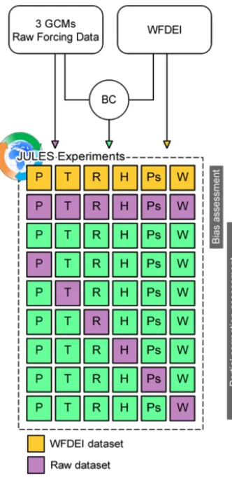
In order to examine the effect of each forcing variable’s bias on runoff we designed and implemented an experiment com-prised of two parts (bias assessment and partial correction bias assessment) and nine sets of JULES’ runs in total. A graphical description of the performed experiment is shown in Fig. 2. Climate data from three GCMs and the WFDEI dataset are used as JULES’ forcing. The sets of runs forced with GCM data include three model runs – one per GCM. Then the analysis progresses using the ensemble mean. The time span of this analysis is the historical period 1981–2010. This is also the time span of the period used for bias correc-tion of the GCM output.
2.7 Bias assessment
The first part of the experiment is to assess initial and re-maining biases in the forcing data and in simulated runoff. Initial bias refers to the difference between raw GCM vari-ables and the respective WFDEI varivari-ables. Remaining bias is the bias in the forcing variables after the bias correction, i.e. the difference between bias corrected GCM variables and the respective WFDEI variables. Referring to runoff, “initial” and “remaining” biases are defined as the difference between runoff simulations forced with raw and bias corrected forc-ing respectively from simulations forced with the WFDEI dataset. This definition is employed to shorten and simplify the expressions used in this paper (i.e. “initial bias in runoff” instead of “the difference between runoff forced with raw GCM data and WFDEI data”). In this part of the experiment, three sets of JULES’ runs were conducted:
i. forced with WFDEI (WFDEI);
[image:4.612.48.547.336.451.2]Figure 2.Graphical description of the performed experiment.
iii. forced with bias corrected climate data (BC). 2.8 Partial correction bias assessment
For the second part of the experiment – the partial correction bias assessment – six more sets of JULES’ runs were per-formed. In each of these runs, one of the six forcing variables (precipitation, temperature, radiation, humidity, surface pres-sure, and wind speed) is used in its raw form, while the rest of the input forcing is bias corrected. The partial correction as-sessment runs are symbolized as NobcV (NOt Bias Corrected variableV), whereV is one of the six forcing variables: pre-cipitation (P), temperature (T), radiation (R), specific hu-midity (H), surface pressure (Ps), and wind (W). It has to be noted here that downward longwave radiation (Rl) and down-ward shortwave (Rs) were examined together; hence, in the respective NobcR run, both downward shortwave and down-ward longwave radiation were forced in uncorrected form. Partial correction assessment is composed as a tool to quan-tify the individual effect of each forcing variable on runoff, but is not designed to suggest and assess run formats.
The simulated runoff of each partially corrected input is compared to the respective simulation in which all input vari-ables are bias corrected (denoted as BC). This comparison allows us to assess the “loss” of the performance of simula-tions when a variable is neglected from the bias correction procedure. It must be noted however that the “loss of perfor-mance” concept bears the assumption that the BC simulation is closer to the WFDEI simulation compared to a partially corrected set.
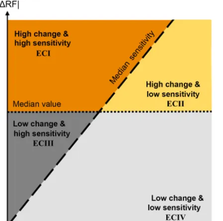
2.9 Categorization of individual variable bias effects A new framework for the classification of the effects of forc-ing variables’ biases on modelled runoff is developed and implemented. The classification employs the comparison of the bias in each forcing variable (1V) and the correspond-ing relative effect in simulated runoff (1RF), discretizing four different categories (Fig. 3). To facilitate the compari-son among the different forcing variables,1V and1RF are expressed as percentages. More specifically,1V and1RF are defined as follows.
1V is the difference between the raw and bias corrected variable value, divided by the bias corrected variable value. 1V is estimated by Eq. (3).
1V =raw variable−BC variable
BC variable ·100 % (3)
As an exception, for temperature1V refers to the abso-lute difference between raw and bias corrected temperature (in K).
1RF expresses the effect of a variable’s bias on runoff and is calculated from the difference between runoff forced with all bias corrected variables except for the examined vari-able V (NobcV) and runoff forced with all bias corrected variables (BC), divided by the runoff of all bias corrected variables (BC).1RF is estimated by Eq. (4).
1RF=RF from NobcV−RF from BC
RF from BC ·100 % (4)
Sensitivity of runoff to changes in forcing variables (S) is the fraction of runoff change over the forcing variable change and serves as a measure to assess the relative magnitude of 1RF compared to1V. When1RF is sensitive to1V, rela-tively smaller changes in the variable should cause relarela-tively larger changes in runoff and vice versa. Sensitivity is in gen-eral dimensionless, but for temperature has units of K−1.S is estimated by
S=1RF/1V . (5)
Figure 3.Categorization of the effect of changes in forcing vari-ables (V) on runoff (RF). The four areas correspond to the four de-fined effect categories. Thexaxis corresponds to relative changes in forcing variables and theyaxis to relative changes in runoff. For all changes, the absolute value is considered.
As shown in Fig. 3, the effect of each variable’s bias (|1V|) on runoff (|1RF|) is separated into four different categories according to two rules. The first rule is the char-acterization of |1RF| among all the experiments as “low” or “high” relative to its median value, shaping the ordinate y=median(|1RF|). Median(|1RF|) is derived considering the |1RF|values of all land grid boxes and for all the ex-periments. The second rule is the characterization of sensi-tivity |S| as high or low relative to its median value. The latter forms a bisectrix s=median(|S|). Median(|S|) is, ac-cordingly to median(|1RF|), derived from the|S|values of all grid boxes and for all the experiments apart from tem-perature. In the case of temperature, median(|S|) is explicitly recalculated from the values of all the land grid boxes of this specific experiment. These two rules form the four categories of Fig. 3. Combinations of the two rules result in four differ-ent effect categories (ECs) presdiffer-ented in decreasing order of the effect of a variable’s bias on runoff:
i. High change and high sensitivity (ECI); ii. high change and low sensitivity (ECII); iii. low change and high sensitivity (ECIII); and
iv. low change and low sensitivity (ECIV). 2.10 Regional-scale bias assessment
Regional focus is given in 24 regions and 9 hydrological basins. The regions were selected from the 26 regions
pre-Table 2. 24 regions of the globe, selected from Giorgi and Bi (2005).
Region name Abbreviation
North Europe NEU
Mediterranean Basin MED
Northeast Europe NEE
North Asia NAS
Central Asia CAS
Tibet TIB
Eastern Asia EAS
Southeast Asia SEA
Northern Australia NAU
Southern Australia SAU
Sahara SAH
Western Africa WAF
Eastern Africa EAF
East Equatorial Africa EQF
South Equatorial Africa SQF
Southern Africa SAF
Western North America WNA
Central North America CNA
Eastern North America ENA
Central America CAM
Amazon AMZ
Central South America CSA
Southern South America SSA
South Asia SAS
sented in Giorgi and Bi (2005) (in our study Alaska and Greenland are excluded from the analysis). The hydrolog-ical basins were selected to cover different hydro-climatic regimes, in conjunction with GRDC data availability. The se-lected regions and basins are shown in Fig. 1. The abbrevia-tions of the regions’ names can be found in Table 2.
3 Results and discussion
3.1 Long-term annual biases in forcing variables at the global scale
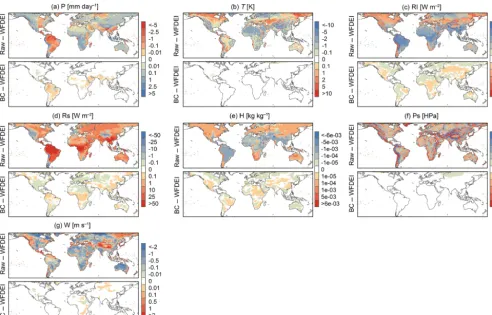
[image:6.612.347.509.97.382.2]Figure 4. Difference maps, showing initial (raw-WFDEI) and remaining (BC-WFDEI) biases of the GCM ensemble forcing variables:
(a)precipitation,(b)temperature,(c)longwave downward radiation,(d)shortwave downward radiation,(e)specific humidity,(h)surface pressure, and(g)wind. Differences are calculated between the long-term annual averages (ANN) of the 1981–2010 period.
to 0.01 mm day−1in absolute terms, for 80.32 % of the land surface) and located in the tropics. The initial biases in tem-perature are cold biases for 57.82 % of the land surface, while warm biases (mainly found in the Alaskan, Greenland, and northern and central Asia regions, as well as in the Mediter-ranean and the Andes) occupy 42.12 % of the land surface (Fig. 4b). Initial biases greater than 2 K in absolute terms cover approximately one-third of the land surface (34.74 %). After bias adjustment, the remaining temperature bias is less than 0.1 K for the vast majority of the land surface (97.27 %). The initial biases of longwave and shortwave radiation (Fig. 4c and d respectively) exhibit similar spatial variations but have different signs. Shortwave radiation shows a greater extent of large biases (> 50 W m−2 in absolute terms) com-pared to longwave radiation (8.16 % as opposed to 2.95 % of the land surface). Initial biases in specific humidity are greater than 10−3kg kg−1 (1 g kg−1), in absolute terms, for one-quarter of the land surface (23.65 %) (Fig. 4e). The largest biases in surface pressure (> 50 or <−50 HPa) occupy 10.01 % of the land surface and are found in the areas where high mountain ranges are located (Rocky Mountains, Andes, Himalayas) (Fig. 4f). The remaining bias in surface pressure is less than 0.1 HPa (in absolute terms) for most of the land
surface (96.50 %). For more than half of the land surface (55.79 %), the wind’s initial biases are larger than 0.5 m s−1 or smaller than−0.5 m s−1(Fig. 4g). The remaining biases of the wind variable range between−0.01 and 0.01 m s−1for the majority of the land surface (87.71 %).
elevation model. Although GCM surface pressure is inter-polated to the WFDEI resolution, this does not correct the elevation-induced error in the GCM simulations.
The remaining biases in precipitation in the tropical re-gions were also identified and discussed extensively by Gril-lakis et al. (2013) and are related to the error in the CDF approximation during bias correction. For the rest of the vari-ables, the remaining bias, although not actually zero, is very close to zero (well below the smallest positive and above the smallest negative rank in the legend, e.g. below−0.1 K and below 0.1 K for temperature). The colour scale in Fig. 4 was selected with the intention of showing the remaining biases, but this does not mean that their values are accountable. They are rather trace errors occurring due to truncation numerical errors during the bias correction process. Hence the remain-ing biases (except for precipitation) could not be attributed to a specific mechanism.
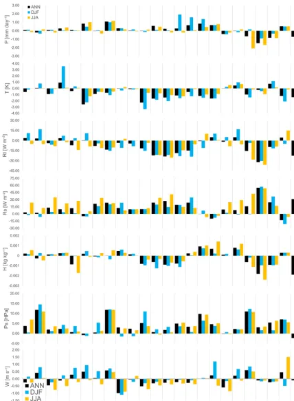
3.2 Regional and seasonal biases in forcing variables Figure 5 illustrates the initial biases of the GCM ensemble, spatially aggregated over 24 regions of the globe. To account for possible seasonality variations, the biases are calculated for the annual mean (ANN) and for the December–January– February (DJF) and June–July–August (JJA) means. The re-maining biases are not shown because their regionally aggre-gated values are negligible and would be indistinguishable in the figure. Additionally, an insight into the behaviour of each ensemble member, in comparison to the ensemble mean and WFDEI, is given by Table S2. Table S2 provides the values of raw input variables for each ensemble member, the ensem-ble mean value, and the respective WFDEI value, averaged for the 24 study regions.
Precipitation biases are less pronounced in Europe (NEU, MED, and NEE) and in central and northern Asian regions (CAS and NAS). The wettest precipitation biases are encoun-tered in equatorial and southern Africa (EQF, SQF, and SAF) and concern DJF precipitation (Fig. 5). The driest biases are found for the CAM, AMZ, and SAS regions, for JJA precip-itation. Temperature displays cold biases in most regions. A notable exception is the warm bias in DJF temperature in the NAS region, which is the most pronounced temperature bias found. Generally the DJF temperature biases are the largest, followed by ANN, while the JJA season has the smallest tem-perature biases.
The two radiation components, longwave (Rl) and short-wave (Rs) radiation, show an inverse behaviour in their bi-ases (Fig. 5). That is to say, in regions where Rl has negative biases, Rs exhibits positive biases and vice versa. According to Demory et al. (2014), overestimation of shortwave radia-tion is a common issue amongst the GCMs. Negative biases are dominant for Rl, in contrast to the Rs variable, which mostly shows positive biases. Specific humidity has negative biases over the northern part of the African continent (SAH, WAF, EAF, and EQF), Central and South America (CAM,
AMZ, and CSA), and South Asia (SAS). Positive humidity biases are identified in the southern part of Africa (SQF and SAF) and North America (WNA, CNA, and ENA).
Surface pressure shows almost exclusively positive biases (Fig. 5). The regions that distinguish for the largest biases are MED, SEA, SAH, SAF, CAM, CSA, and SSA. The most dominant negative wind speed bias is found in NAU. Most of the African continent (SAH, WAF, EAF, EQF, and SQF) and of South America (AMZ and CSA) also have negative biases in wind. The largest positive biases are encountered in the southern part of South America (SSA) for the JJA season and for the DJF season in regions of North America (WNA and CAM), Europe (MED), and Asia (CAS, TIB, and SEA). 3.3 Model evaluation
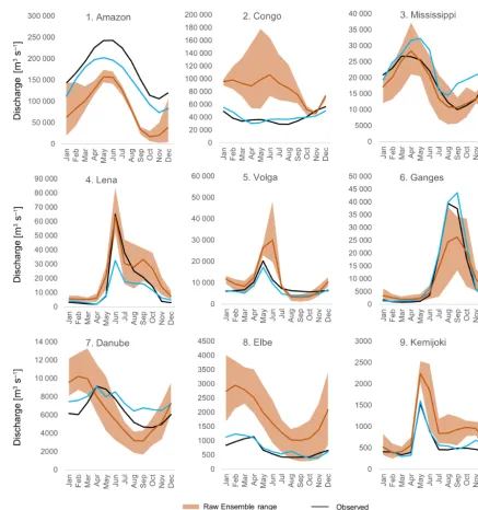
In order to assess JULES’ performance, we compare dis-charge modelled with WFDEI and with the raw GCM dataset to discharge observations for nine study basins. Figure 6 shows the seasonality of observed and modelled discharge and the evaluation metrics of the two sets of simulations (WFDEI and raw GCM) are presented in Table 3.
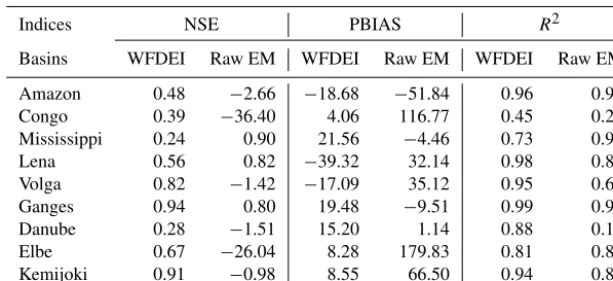
For seven out of the nine basins (Amazon, Congo, Volga, Ganges, Danube, Elbe, and Kemijoki) seasonality is captured well by the WFDEI simulation (Fig. 6). In contrast, the raw GCM simulation exhibits significant positive and negative bi-ases for these seven basins. For the two remaining basins, however (Mississippi and Lena), seasonality is better cap-tured by the raw GCM simulation. The WFDEI run results in positive NSE values (0.24 to 0.94) for all the basins. By contrast, the raw GCM run results in negative NSE values for six out of the nine basins. PBIAS indicates that the raw GCM simulation exhibits greater deviations from observa-tions than the WFDEI run for most basins (excepobserva-tions are the Mississippi, Lena, Ganges, and Danube). Finally, theR2 metric shows that the linear correlation between simulations and observations is stronger for the WFDEI run for seven out of the nine basins (exceptions are the Mississippi and Elbe). For both simulations the lowestR2value is reported for the Congo basin (0.45 and 0.2 for the WFDEI and raw GCM runs respectively). The best correlations per simulation are found for the Ganges for the WFDEI run (0.99) and for the Amazon for the raw GCM run (0.94).
Table 3.Evaluation metrics derived from monthly discharge data. Metrics are calculated for JULES’ simulations from WFDEI data (WFDEI) and the ensemble mean of raw GCM data (raw EM).
Indices NSE PBIAS R2
Basins WFDEI Raw EM WFDEI Raw EM WFDEI Raw EM
Amazon 0.48 −2.66 −18.68 −51.84 0.96 0.94
Congo 0.39 −36.40 4.06 116.77 0.45 0.20
Mississippi 0.24 0.90 21.56 −4.46 0.73 0.92
Lena 0.56 0.82 −39.32 32.14 0.98 0.89
Volga 0.82 −1.42 −17.09 35.12 0.95 0.66
Ganges 0.94 0.80 19.48 −9.51 0.99 0.91
Danube 0.28 −1.51 15.20 1.14 0.88 0.19
Elbe 0.67 −26.04 8.28 179.83 0.81 0.86
Kemijoki 0.91 −0.98 8.55 66.50 0.94 0.89
error component, which is not considered here, could result from the uncertainty in discharge measurements (Coxon et al., 2015).
The model evaluation has revealed two basins (Missis-sippi and Lena) for which raw GCM forced discharge sim-ulations outperform the WFDEI simsim-ulations. For the Missis-sippi, the WFDEI run gives higher discharge than the ob-servations throughout the year, revealing a deficiency of the model in capturing the water balance of this basin. Most of the Mississippi extent is in the CNA region, where negative precipitation biases have been documented (Fig. 5). Thus, the raw GCM run is forced with less precipitation compared to WFDEI and less discharge is produced, masking the model deficiency in this basin and improving the metrics of model performance. It is also important to note that the range of the raw GCM simulations is quite broad, especially for a three-member ensemble. The upper range of the GCM ensemble exceeds the WFDEI-simulated runoff during almost half the seasonal cycle. This indicates that the individual ensemble members would not necessarily outperform the WFDEI run and that, for this specific basin, the ensemble averaging has possibly produced a “false positive” in model performance. In this particular basin, model performance may also be hin-dered due to the comparison of naturalized and actual dis-charge, as the Mississippi is a heavily regulated river. For the Lena, the WFDEI run underestimates measured discharge by about 40 %. The Lena basin falls into the extent of the NAS region, for which positive precipitation biases have been doc-umented (Fig. 5). The extra water in the raw GCM run coun-teracts the tendency of the model to underestimate discharge in the Lena basin, resulting in an improved model perfor-mance. In the context of the present study we are not able to identify the exact reasons why model performance is hin-dered in some basins. It is unrealistic for a global LSM to achieve top performance around the world (Hattermann et al., 2017), as, due to its global nature, some fixes in some regions could result in deteriorations in performance in other parts of the land surface. Thus, the interpretation of the following
analysis of the present study should consider the model defi-ciencies revealed in this section.
3.4 Long-term biases in runoff at the global scale Figure 7 shows the initial and remaining biases in runoff, de-rived from ANN, DJF, and JJA long-term means. As with the biases in the input forcing variables, the remaining bias in runoff is 1 to 2 orders of magnitude smaller than the ini-tial bias. Hence, the use of bias corrected data led to an im-proved representation of runoff by the model, compared to the baseline of the WFDEI run. Accordingly, the studies of Teutschbein and Seibert (2012) and Rojas et al. (2011) found that hydrological simulations are substantially improved with the use of bias corrected forcing.
Regarding the raw GCM run, the largest runoff underes-timation biases (<−5 mm day−1) are encountered in Central and North America, the central–eastern part of South Amer-ica, and East Asia. The most pronounced runoff overestima-tion biases are found in the western part of North and South America, in equatorial and southern Africa, northern Europe, the Tibetan region, and Indonesia. Initial runoff biases are larger than 1 mm day−1in absolute terms for 16.26, 14.85, and 20.18 % of the land surface respectively for ANN, DJF, and JJA. The differences between the seasonal means (DJF, JJA) and the annual mean (ANN) are in general subtle. How-ever, the increases in runoff overestimation biases in DJF in southern equatorial Africa and in JJA in the Tibetan plateau are worth noting. Large initial biases (> 5 mm day−1in ab-solute terms) in seasonal means occupy a greater percentage of the land surface compared to the annual mean (0.70 % for ANN, compared to 1.25 and 1.97 % for DJF and JJA respec-tively).
Figure 6.Discharge seasonality (m3s−1) derived from the period 1981–2010 for nine study basins. Each panel shows observed discharge (GRDC measurements) compared to JULES’ simulated discharge from WFDEI data and raw GCM data (the mean and the range of the ensemble are shown).
for DJF, and 34.42 % for JJA). The (negative) remaining bias in ANN runoff is more pronounced in the western Amazo-nian region. This probably corresponds to the remaining bias in precipitation identified for the Amazonian region (Fig. 4). In addition to the significant reduction of the biases in runoff forced with bias corrected data, it can be observed that the remaining biases have switched signs compared to the ini-tial biases. This means that in regions where the iniini-tial bias in runoff is positive (negative), the raw GCM forced runoff is larger (smaller) than runoff forced with WFDEI, and the use of bias corrected forcing results in runoff slightly lower
Figure 7.Runoff (mm day−1) from WFDEI data (left column). Initial (raw-WFDEI) and remaining (BC-WFDEI) biases in runoff are shown in the middle and right columns respectively. Results are shown for long-term annual averages (ANN) and for December–January–February (DJF) and June–July–August (JJA) averages of the 1981–2010 period.
3.5 Effect of each forcing variable’s bias on runoff The effect that the bias of each forcing variable can have on runoff is investigated here, by comparing runoff from the bias corrected run to the partial correction assessment runs. The results are shown in Fig. 8, for ANN, DJF, and JJA averages. First, we discuss the runoff differences calculated from the ANN period. Precipitation and temperature are the only two variables that cause runoff differences larger than 5 mm day−1 (in absolute terms) when neglected from bias correction. However, these differences regard a very small percentage of the land surface: 0.61 % for precipitation and only 0.02 % for temperature. Moreover, precipitation bias causes changes in runoff greater than 1 mm day−1(in abso-lute terms) for 14.28 % of the land area. Such changes for the other variables occupy a significantly smaller fraction of the land area (ranging from 1.21 % for temperature to 0.05 % for wind). Based on the above it can be stated that precipitation is the variable that most affects runoff response. Precipita-tion bias causes both wet and dry biases in different regions of the land surface, with a pattern that closely resembles the effect of the initial GCMs’ biases on runoff (Fig. 7). A similar pattern between precipitation and runoff biases was also ob-served by Teng et al. (2015), who noted that precipitation er-rors are magnified in modelled runoff. Temperature biases re-sult in runoff overestimation for around 60 % of the land sur-face (e.g. over western and eastern North America, the Ama-zon region, equatorial Africa, northern Europe, and parts of Asia) and runoff underestimation for around 40 % (example
regions: parts of Central and South America and of central Asia). Temperature biases correspond to small changes in runoff (up to 0.01 mm day−1 in absolute terms) over about one-third of the land area. Excluding the radiation compo-nents from the bias correction procedure produces negative runoff changes for the majority of the land surface (67.60 %), while for around 80 % of the land surface the differences in runoff range between−0.1 and 0.1 mm day−1. The bias in the specific humidity variable corresponds to runoff overes-timations for 64 % of the land area. The areas of runoff over-estimation are mainly located at the higher latitudes (north-ern part of North America, Europe, and north(north-ern Asia). For 36.43 % of the land surface, changes in runoff due to specific humidity biases span between 0.1 and 0.5 in absolute terms. Surface pressure and wind are the variables that show the smaller effect on the hydrological output, as their exclusion from bias correction corresponds to small changes in runoff (less than 0.1 mm day−1in absolute terms) for the vast ma-jority of the land surface (around 94 and 92 % of the land sur-face respectively for sursur-face pressure, and wind speed). The most pronounced differences in runoff due to surface pres-sure biases are negative and are encountered over the high mountain range regions of South America and Asia (Andes and Himalayas respectively).
to the seasonal values, with small variations on the land frac-tions that show a specific response to forcing biases.
From this analysis it can be deduced that apart from the main hydrological cycle drivers (precipitation and temper-ature), radiation and specific humidity can also have a sub-stantial effect on runoff, especially for specific regions. These findings will be further investigated and discussed in the fol-lowing sections. Other studies also advocate the considerable effect that biases in radiation (Mizukami et al., 2014) and hu-midity (Masaki et al., 2015) can have on hydrological fluxes. 3.6 Runoff sensitivities to forcing variables
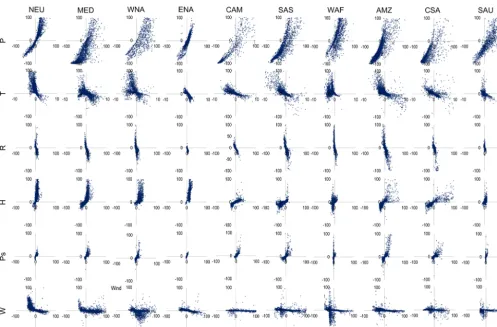
Sensitivity of runoff changes to the biases of the forcing vari-ables is examined by exploring the relationship between the input forcing biases (1V) and the corresponding changes in runoff (1RF). The regional variation of this relationship is also investigated. Figure 9 shows scatterplots of1RF versus 1V for each examined variable, for 10 selected regions. The dots in each scatterplot correspond to the land grid boxes of each region. The presented regions are selected as represen-tative of different parts of the land surface, as the number of the regions shown in the manuscript had to be reduced for clarity of the results. Scatterplots of the 24 examined regions can be found in the Supplement of this paper (Fig. S3). The median values of 1V, 1RF, andS of the land grid boxes of each region, for the 24 examined regions, are shown in Table 4.
The correlation between the six1Vs and respective1RFs differs substantially between the examined regions. Gener-ally, the correlations show a non-uniform behaviour, identi-fied by the highly scattered data clouds. This implies a high spatial variability of runoff sensitivity to the examined vari-ables.
For precipitation, the1RF over1P relationship exhibits a non-linear behaviour, indicating that the relative change in runoff is not proportional to precipitation bias, but also depends on the magnitude of precipitation bias. Renner et al. (2012) also identified non-linearities in the relationship between relative changes in streamflow and changes in pre-cipitation, and argued that non-linear behaviour is a result of the combined effects of water and energy balances. Temper-ature biases have an inversely proportional and highly non-linear relationship with changes in runoff. The1RF over1T relationship is also variant for different regions. For example, the scatterplots for NEU and WNA indicate that small tem-perature biases may correspond to large changes in runoff. In contrast, the scatterplot for CAM indicates that larger temperature biases correspond to smaller changes in runoff compared to the other regions. Radiation biases are small but can correspond to high changes in runoff for some re-gions (WNA, SAS, WAF, and AMZ). For specific humidity it can be observed that small positive biases correspond to high changes in runoff for some regions (NEU, MED, WNA, and ENA). A different behaviour is observed for CAM, SAS,
AMZ, and CSA, where the data cloud is more scattered on thex axis (meaning larger biases in specific humidity) and less scattered on they axis (i.e. changes in runoff are smaller). Surface pressure has smaller biases compared to the other forcing variables and its effect on runoff also ap-pears reduced. Wind has a wide range of both positive and negative biases which, however, do not seem to affect runoff accordingly.
The variation of the1RF over 1V relationships across the different regions can be attributed to a number of factors. First, it depends on the magnitude and signal of the biases in the forcing variables. As previously shown, these can have significant spatial variations (Fig. 4). For example, according to the median values of relative changes in Table 3, some re-gions are dominated by negative precipitation biases (MED, SAS, AMZ, and CSA) and others by positive biases (NEU, WNA, ENA, CAM, WAF, and SAU). Second, it reflects the climatology of each region. The same biases would affect differently regions with different runoff (and evapotranspira-tion) fractions of each region. The precipitation partitioning to runoff and evapotranspiration is a climate characteristic and is controlled by either water or energy limitations, de-pending on the region. Additionally, we should consider that although we assess the effect of long-term annual biases on long-term annual runoff, the results are still dependent on the seasonal cycles of the variables and/or runoff, especially if the seasonality of precipitation in the region is strong. For example, the same annual bias in temperature would trans-late differently to runoff changes in a region with precipita-tion evenly dispersed throughout the year and in another re-gion where most of the annual precipitation happens during the summer months. Finally, as this is a model-based experi-ment, we should consider whether high sensitivities of some variables for specific regions are a result of over-sensitivity of the model. Vano et al. (2012) documented considerable differences in the spatial distribution of sensitivities to pre-cipitation modelled by five LSMs.
3.7 Spatial distribution of bias effect categories
Figure 10 shows global maps of bias ECs for each forcing variable, derived according to the methodology described in Sect. 2.8. The land area fraction corresponding to each EC is tabulated in Table 5.
Figure 9.Scatterplots of relative changes in the forcing variable (1V,xaxis) and corresponding relative changes in runoff (1RF,yaxis), for all the forcing variables and for selected regions. In each panel, each dot represents the1RF/ 1V relationship of each land grid box in the examined region.
show a significant spatial coherence and are clustered at the higher latitudes of the globe. Surface pressure biases belong to ECI for around one-tenth of the land surface. The highly affected areas mainly correspond to regions with high moun-tain ranges. For wind the majority of the land surface corre-sponds to ECIV. Still, around one-quarter of the land surface belongs to the high change categories (ECI and ECII). 3.8 Discussion of runoff sensitivities
Here we compare our findings to the respective literature to assess the realism of JULES’ sensitivity. We use the median sensitivity value of the grid boxes of each region (Table 4) as the representative sensitivitySfor each region. Moreover, we discuss issues of possible model over-sensitivity in particular regions and the caveats of this study.
3.8.1 Sensitivity of runoff to precipitation
Most studies have examined the sensitivity (also reported as elasticity) of runoff (or discharge) to precipitation. A num-ber of studies have examined sensitivity to precipitation for regions or basins in the United States. Values of runoff
Table 4.Relative change (%) in forcing variable (1V), corresponding relative change (%) in runoff (1RF), and sensitivities (S=1RF/1V) per region, for each variable. For each region, the median of the1V,1RF, andSvalues of all land grid boxes is shown.
Variables P T∗ R H Ps W
GLOBAL 1V 14.46 −0.57 1.73 0.91 −0.02 −5.86
1RF 2.49 3.38 −3.71 2.04 −0.04 0.21 S 1.76 −0.05 −2.12 0.81 1.18 −0.06
NEU 1V 14.6 −0.46 1.86 4.1 −0.05 −9.79
1RF 27.97 22.68 −5.25 25.49 −0.02 3.62
S 2.10 −0.31 −3.31 5.24 2.90 −0.36
MED 1V −14.39 −0.15 0.55 −1.34 0.41 14.94
1RF −58.56 1.55 −1.51 4.07 0.44 −0.47
S 2.02 −0.04 −2.52 0.77 1.08 −0.08
NEE 1V 4.89 −1.44 2.44 3.32 0.1 −11.77
1RF 5.75 47.11 −5.39 32.73 0.26 5.98
S 2.28 −0.32 −2.64 9.58 3.31 −0.50
NAS 1V 26.05 0.67 3.53 8.05 −0.06 −1.08
1RF 59.36 11.8 −10.08 63.98 0.02 4.06
S 2.35 −0.07 −2.95 7.58 2.43 −0.29
CAS 1V 6.44 −0.03 1.37 −13.00 −0.41 8.09
1RF −9.94 1.31 −0.44 −0.19 −0.36 −1.29 S 2.49 −0.05 −3.50 0.31 0.88 −0.09
TIB 1V 128.47 −2.94 −1.14 7.69 −0.12 12.59
1RF 1017.17 5.38 0.97 0.81 0.02 0.06
S 7.27 −0.02 −2.07 0.18 0.40 0.00
EAS 1V 19.25 −0.94 2.51 2.92 −0.2 −3.55
1RF 4.36 5.54 −2.96 3.66 −0.05 0.76 S 1.70 −0.06 −1.53 0.82 1.07 −0.09
SEA 1V 19.76 −0.87 1.11 0.89 0.23 34.57
1RF 43.92 5.97 −3.2 1.66 0.32 −1.04
S 2.07 −0.08 −2.68 1.16 1.54 −0.05
NAU 1V 41.15 −0.04 1.43 7.71 0.1 −28.46
1RF −5.13 1.02 −1.16 1.38 0.09 −0.44 S 0.37 −0.03 −0.75 0.31 0.56 0.00
SAU 1V 18.92 −0.28 0.85 2 −0.13 −11.2
1RF −9.29 1.07 −0.11 1.4 0.06 −0.49 S 0.82 −0.05 −0.88 0.67 1.00 −0.03
SAH 1V 54.11 −2.73 −0.47 −8.96 0.22 −13.59
1RF −2.59 −0.68 0.64 −0.32 0 0.08 S 0.94 0.00 −0.25 0.04 0.04 −0.01
WAF 1V 26.74 −1.51 −0.88 −5.79 −0.1 −15.13
1RF 58.24 5.61 −1.57 −0.71 −0.13 0.09
S 2.78 −0.04 −2.61 0.22 1.28 −0.04
EAF 1V 23.22 −1.68 −0.06 −5.76 −0.25 −12.11
1RF 42.13 7.24 −1.51 −3.74 −0.28 0.09
S 2.12 −0.05 −1.95 0.48 0.95 0.00
EQF 1V 5.64 −1.55 −0.25 −2.15 −0.2 −10.09
Table 4.Continued.
Variables P T∗ R H Ps W
SQF 1V 36.45 −0.9 0.9 0.89 −0.03 −15.6
1RF −73.18 −82.26 −85.07 −84.68 −84.2 −84.18
S 2.94 −0.07 −1.91 0.59 1.10 −0.04
SAF 1V 89.8 −1.41 −0.38 14.28 0.68 −4.74
1RF 85.47 5.5 0.54 5.33 0.42 −0.02
S 1.35 −0.04 −1.66 0.45 0.72 −0.05
WNA 1V 65.92 −1.75 −1.23 13.55 0.14 10.23
1RF 112.66 17.94 −0.48 9.85 0.16 −2.5
S 2.12 −0.13 −2.01 0.77 0.98 −0.17
CNA 1V −12.84 0.11 1.68 2.29 −0.08 −14.79
1RF −50.86 1.53 −2.06 6.57 −0.05 1.96
S 2.54 −0.07 −1.47 1.08 1.09 −0.13
ENA 1V 4.08 0.49 2.71 13.4 0.1 5.47
1RF −0.38 −0.38 −5.18 39.72 0.13 0.86
S 1.69 −0.07 −1.92 3.17 1.54 −0.11
CAM 1V 11.43 −0.98 −0.4 −6.16 0.15 25.27
1RF −7.73 3.65 −0.1 −2.55 0.14 −0.52 S 1.32 −0.04 −1.58 0.49 0.77 −0.02
AMZ 1V −26.58 −0.35 4.06 −13.19 −0.19 −4
1RF −40.52 4.88 −9.34 −6.01 −0.23 0.03
S 1.42 −0.05 −2.37 0.53 1.44 −0.04
CSA 1V −32.8 0.7 3.05 −11.53 −0.23 −7.5
1RF −63.21 −1.49 −3.22 −5.75 −0.13 0.38
S 1.59 −0.04 −1.16 0.53 0.83 −0.04
SSA 1V 72.07 −1.22 −1.77 5.07 0.08 9.91
1RF 84.32 10.06 −0.47 12.05 0.34 −2.44
S 1.53 −0.09 −0.50 1.48 1.29 −0.04
SAS 1V −9.19 −1.08 1.39 −13.11 −0.05 −6.81
1RF −26.35 5.2 −4.07 −2.53 −0.09 0.51
S 1.62 −0.05 −2.46 0.29 0.90 −0.05
*1Vfor temperature is the absolute change in temperature.
Table 5.Percent of land area (%) under each of the four effect cat-egories (ECs).
Variables/ I II III IV
ECs
P 67.80 24.20 1.82 6.18
T 45.15 22.03 2.46 30.35
R 48.74 1.30 26.16 23.80
H 40.80 13.76 5.58 39.86
Ps 12.17 1.83 38.48 47.52
W 6.09 19.19 2.35 72.37
agreement with the literature (S to precipitation for EAS is 1.70).
3.8.2 Sensitivity of runoff to temperature and other variables
[image:17.612.78.256.561.660.2]sensitiv-Figure 10.Global maps of bias effect categories (ECs) for each forcing variable.
ities by perturbing daily temperature maxima and minima. These changes also affect the downward longwave radiation and humidity, which are then used by the evapotranspiration routines of the LSMs. In our case, the change in temperature does not interact with radiation and humidity, as those are read as input variables by the model. When temperature is allowed to interact with humidity, increased temperature will increase the water vapour capacity of the air, and more wa-ter will be evaporated. The lack of this physical link in our simulations could, to an extent, explain the decreased sen-sitivity of runoff to temperature changes compared to Vano et al. (2012). In the analysis of Brikowski (2015), sensitiv-ities of runoff to precipitation and temperature are derived from the respective historical data. Thus, sensitivity to tem-perature will also include the changes caused by the interac-tion of temperature with other meteorological variables. In a study with a different approach, Yang and Yang (2011) sep-arated the effect of precipitation, temperature, net radiation, relative humidity, and wind speed on runoff and calculated sensitivities for each variable. They reported values of Sto temperature ranging from −0.11 to−0.02 C−1between 89 catchments of the EAS region. For the same region, we have computedSto temperature as−0.06 K−1, which is included in the stated range in the literature. Moreover, our S
val-ues for radiation, humidity, and wind speed are also in good agreement with Yang and Yang (2011). According to Yang and Yang (2011),S to radiation ranges from−1.9 to−0.3, S to humidity from 0.2 to 1.9, and S to wind speed from
−0.8 to−0.1. The range refers to values computed for 89 catchments in the EAS region. Our respective values for this region are−1.53 for radiation, 0.82 for humidity, and−0.09 for wind speed. This supports the argument that the large de-viations of the sensitivity to temperature between our study and the studies of Vano et al. (2012) and Brikowski (2015) result from interactions in the forcing variables included in the referenced studies.
3.8.3 Sensitivity of runoff to radiation
[image:18.612.50.547.64.384.2]Figure 11. (a)Latitudinal means of raw and bias corrected specific humidity (g kg−1),(b)latitudinal means of JULES’ runoff forced with raw and bias corrected specific humidity (mm day−1), and
(c)percent differences of the latitudinal means in(a)Hand(b)RF. The latitudinal means are calculated from the 1981–2010 period.
the two radiation components have inverse signs for most re-gions (Fig. 5).
3.8.4 Sensitivity of runoff to specific humidity in high-latitude regions
AlthoughSto humidity for EAS compares well with the lit-erature, unexpectedly high values ofSto humidity are found for other regions (5.24 for NEU, 9.58 for NEE, and 7.58 for NAS). We performed an extra analysis to investigate this is-sue and the basic findings are included in Fig. 11 and the Supplement of this paper. Figure 11 examines the differences between the latitudinal mean of raw and bias corrected spe-cific humidity and the resulting runoff. Very high sensitiv-ity of runoff to H is observed for a specific area, the zone between 70 and 40◦N latitudes. In that zone, a difference of about 10 % in H corresponds to an increase of 40 to 60 % in runoff. Investigation of the different fluxes related to runoff production in the model revealed two mechanisms
that explain this behaviour. First, due to higher humidity, the water vapour deficit of the air is reduced and evapotranspi-ration is decreased, thus allowing more of the precipitated water available as runoff. This mechanism explains around one-third of the magnitude of reported changes in runoff (Fig. S4). The second mechanism happens due to supersat-uration of the air, especially during the colder months of the year when the dew point is lower, and includes the con-densation and deposition of water vapour (direct transition from vapour to ice). Depositioned water accumulates as snow mass. Snow mass is higher for the rawH run (H has posi-tive biases), which results in increased snowmelt and thus increased runoff (Fig. S5).
A comparison of supersaturated air conditions for the dif-ferent sets of data (WFDEI, raw, BC, and NobcH) can help us identify the origin of the aforementioned behaviour. From the input specific humidityH, we estimated the respective rela-tive humidity (this transformation also requires temperature T and surface pressure Ps as input to the Clausius–Clapeyron equation). Then we calculated the fraction of time (based on a daily time step) in which supersaturated conditions occur, for the historical period 1981–2010. The estimation was per-formed for (a) the WFDEIH,T, and Ps, (b) the rawH,T, and Ps, (c) the bias correctedH,T, and Ps, and (d) for a combination of data corresponding to the NobcH run (rawH combined with bias correctedT and Ps). The results are pre-sented in Fig. 6 of the Supplement of this paper. The analy-sis reveals that the higher-latitude regions – that display high sensitivity of runoff toH – are under supersaturated condi-tions for more than 10 % of the time (Fig. S6). The length of supersaturated conditions estimated for the WFDEI, raw, or BC data do not exhibit a respective spatial pattern, although supersaturation is found in all three datasets (Fig. S6). Thus, the high runoff sensitivity over the high-latitude regions is not a result of supersaturated conditions in the raw GCM H, and it rather stems from (1) raw GCM H being higher than BCHand (2) the calculation of relative humidity within JULES, done by combining raw GCMHwith bias corrected T and Ps. This inconsistency strengthens the argument for the need for bias correction of more forcing variables – in addition toP andT. Specific humidity is a variable that is often left uncorrected, a practice that could possibly result in runoff overestimations at the northern latitudes based on our findings, in cases where hydrological models which account for deposition and condensation are used.
[image:19.612.46.290.66.411.2]3.9 Study caveats
An issue that must be considered for the interpretation of the results of this study is that they have been based on a sin-gle impact model. As the uncertainty stemming from the se-lection of the impact model is large (Gudmundsson et al., 2012; Hagemann et al., 2013), it is preferable to use mul-tiple models in order to capture a wide range of possible re-sults. The effect of the meteorological forcing on a hydrolog-ical output is heavily model dependent, as different models employ different concepts and/or equations for the represen-tation of key hydrological processes. This concern has also been discussed by other single model studies on meteorolog-ical variables’ effects on hydrologmeteorolog-ical outputs (Mizukami et al., 2014; Masaki et al., 2015). Nonetheless, the results of single model studies are useful in giving indicative answers on the issues they examine and set a basis for the methodol-ogy needed for the respective multi-model applications.
4 Summary and conclusions
The present study examined the effect of the biases in GCM output variables on historical runoff simulations, using the JULES LSM. The effects of biases were studied for each forcing variable separately, for a total of six meteorologi-cal variables (precipitation, temperature, radiation, specific humidity, surface pressure, and wind speed). Biases of each variable and the respective effect of runoff were quantified at the global and regional scales. A framework for the catego-rization of the effects of biases of the different variables was developed and implemented, leading to global maps of bias ECs.
We found that bias correction of GCM outputs results in substantially improved representation of historical runoff. For this reason, our study adds to the numerous studies that advocate the use of some kind of bias correction of GCM data prior to their use as impact model forcing. Precipitation and temperature biases were identified as causing the largest changes in runoff. Radiation and specific humidity can also have a substantial effect on runoff, especially for specific re-gions. The sensitivity of runoff to the different forcing vari-ables exhibits a high spatial variability. Depending on the re-gion, runoff can be more sensitive to radiation or humidity compared to precipitation or temperature. The produced EC maps show that all variables can potentially affect runoff to a high extent, depending on the region. The fraction of the land surface occupied by the high effect category ECI (high changes in runoff and high sensitivity of runoff to the vari-able’s changes) ranges between the variables from 67.80 % for precipitation to 6.09 % for wind.
The produced maps of ECs aid the identification of the re-gions most affected by the bias of each variable. Thus, they could serve as a decision tool in cases when an informed de-cision needs to be made on the variables that would need to
be bias corrected or could be neglected from bias correction, according to the planned model application. Moreover, when raw forcing is used in model applications, EC maps could provide guidance towards the areas where the results would need more careful interpretation.
Based on the findings of this study, we suggest that the widely used concept of bias correcting precipitation and tem-perature should be extended to include more input variables. Radiation and specific humidity should be added to the prior-ity variables for bias correction in hydrological applications, along with precipitation and temperature.
Due to the heavily model-dependent nature of runoff sen-sitivity to forcing variables, generalized conclusions for the behaviour of other impact models to GCM biases cannot be drawn from the present single model assessment. Neverthe-less, this study aims to initiate a discussion of the effect of GCM biases on hydrological output, as the consideration of these sensitivities is crucial to understanding the uncertainty spectrum of hydrologically relevant climate change assess-ments.
Data availability. The WFDEI.GPCC datasets treated as obser-vations in the present study were provided in the framework of the ISIMIP project (http://www.isimip.org/) and obtained through the vre2.dkrz.de server. Raw climate model data (IPSL-CM5A, MIROC-ESM-CHEM, GFDL-ESM2M) of the CMIP5 project have been downloaded through the Earth System Grid Federa-tion (ESGF) (https://esgf-node.llnl.gov/search/cmip5/).
The Supplement related to this article is available online at https://doi.org/10.5194/hess-21-4379-2017-supplement.
Competing interests. The authors declare that they have no conflict of interest.
Acknowledgements. We acknowledge the World Climate Research Programme’s Working Group on Coupled Modelling, which is re-sponsible for CMIP, and we thank the climate modelling groups (listed in Table 1 of this paper) for producing and making available their model output. For CMIP the US Department of Energy’s Pro-gram for Climate Model Diagnosis and Intercomparison provides coordinating support and led development of software infrastruc-ture in partnership with the Global Organization for Earth System Science Portals.
The research leading to these results has received funding from the HELIX project of the European Union’s Seventh Framework Programme for research, technological development and demon-stration under grant agreement no. 603864.
Edited by: Stacey Archfield
References
Best, M. J., Pryor, M., Clark, D. B., Rooney, G. G., Essery, R. L. H., Ménard, C. B., Edwards, J. M., Hendry, M. A., Porson, A., Gedney, N., Mercado, L. M., Sitch, S., Blyth, E., Boucher, O., Cox, P. M., Grimmond, C. S. B., and Harding, R. J.: The Joint UK Land Environment Simulator (JULES), model description – Part 1: Energy and water fluxes, Geosci. Model Dev., 4, 677–699, https://doi.org/10.5194/gmd-4-677-2011, 2011.
Blyth, E., Clark, D. B., Ellis, R., Huntingford, C., Los, S., Pryor, M., Best, M., and Sitch, S.: A comprehensive set of benchmark tests for a land surface model of simultaneous fluxes of water and carbon at both the global and seasonal scale, Geosci. Model Dev., 4, 255–269, https://doi.org/10.5194/gmd-4-255-2011, 2011. Brikowski, T. H.: Applying multi-parameter runoff elasticity
to assess water availability in a changing climate: An ex-ample from Texas, USA, Hydrol. Process., 29, 1746–1756, https://doi.org/10.1002/hyp.10297, 2015.
Bromwich, D. H., Otieno, F. O., Hines, K. M., Manning, K. W., and Shilo, E.: Comprehensive evaluation of po-lar weather research and forecasting model performance in the Antarctic, J. Geophys. Res.-Atmos., 118, 274–292, https://doi.org/10.1029/2012JD018139, 2013.
Christensen, J. H., Boberg, F., Christensen, O. B., and Lucas-Picher, P.: On the need for bias correction of regional climate change projections of temperature and precipitation, Geophys. Res. Lett., 35, L20709, https://doi.org/10.1029/2008GL035694, 2008.
Clark, D. B., Mercado, L. M., Sitch, S., Jones, C. D., Gedney, N., Best, M. J., Pryor, M., Rooney, G. G., Essery, R. L. H., Blyth, E., Boucher, O., Harding, R. J., Huntingford, C., and Cox, P. M.: The Joint UK Land Environment Simulator (JULES), model description – Part 2: Carbon fluxes and vegetation dynamics, Geosci. Model Dev., 4, 701–722, https://doi.org/10.5194/gmd-4-701-2011, 2011.
Coxon, G., Freer, J., Westerberg, I. K., Wagener, T., Woods, R., and Smith, P. J.: A novel framework for discharge uncertainty quantification applied to 500 UK gauging stations, Water Resour. Res., 51, 5531–5546, https://doi.org/10.1002/2014WR016532, 2015.
Demory, M. E., Vidale, P. L., Roberts, M. J., Berrisford, P., Strachan, J., Schiemann, R., and Mizielinski, M. S.: The role of horizontal resolution in simulating drivers of the global hydrological cycle, Clim. Dynam., 42, 2201–2225, https://doi.org/10.1007/s00382-013-1924-4, 2014.
Dufresne, J.-L., Foujols, M.-A., Denvil, S., Caubel, A., Marti, O., Aumont, O., Balkanski, Y., Bekki, S., Bellenger, H., Benshila, R., Bony, S., Bopp, L., Braconnot, P., Brockmann, P., Cadule, P., Cheruy, F., Codron, F., Cozic, A., Cugnet, D., de Noblet, N., Duvel, J.-P., Ethé, C., Fairhead, L., Fichefet, T., Flavoni, S., Friedlingstein, P., Grandpeix, J.-Y., Guez, L., Guilyardi, E., Hauglustaine, D., Hourdin, F., Idelkadi, A., Ghattas, J., Jous-saume, S., Kageyama, M., Krinner, G., Labetoulle, S., Lahel-lec, A., Lefebvre, M.-P., Lefevre, F., Levy, C., Li, Z. X., Lloyd, J., Lott, F., Madec, G., Mancip, M., Marchand, M., Masson, S., Meurdesoif, Y., Mignot, J., Musat, I., Parouty, S., Polcher, J., Rio, C., Schulz, M., Swingedouw, D., Szopa, S., Talandier, C., Terray, P., Viovy, N., and Vuichard, N.: Climate change projections us-ing the IPSL-CM5 Earth System Model: from CMIP3 to CMIP5,
Clim. Dynam., 40, 2123–2165, https://doi.org/10.1007/s00382-012-1636-1, 2013.
Dunne, J. P., John, J. G., Adcroft, A. J., Griffies, S. M., Hallberg, R. W., Shevliakova, E., Stouffer, R. J., Cooke, W., Dunne, K. A., Harrison, M. J., Krasting, J. P., Malyshev, S. L., Milly, P. C. D., Phillipps, P. J., Sentman, L. T., Samuels, B. L., Spelman, M. J., Winton, M., Wittenberg, A. T., and Zadeh, N.: GFDL’s ESM2 Global Coupled Climate–Carbon Earth System Models. Part I: Physical Formulation and Baseline Simulation Characteristics, J. Climate, 25, 6646–6665, https://doi.org/10.1175/JCLI-D-11-00560.1, 2012.
Ehret, U., Zehe, E., Wulfmeyer, V., Warrach-Sagi, K., and Liebert, J.: HESS Opinions “Should we apply bias correction to global and regional climate model data?”, Hydrol. Earth Syst. Sci., 16, 3391–3404, https://doi.org/10.5194/hess-16-3391-2012, 2012. Elsner, M. M., Gangopadhyay, S., Pruitt, T., Brekke, L. D.,
Mizukami, N., Clark, M. P., Elsner, M. M., Gangopadhyay, S., Pruitt, T., Brekke, L. D., Mizukami, N., and Clark, M. P.: How Does the Choice of Distributed Meteorological Data Affect drologic Model Calibration and Streamflow Simulations?, J. Hy-drometeorol., 15, 1384–1403, https://doi.org/10.1175/JHM-D-13-083.1, 2014.
Fu, G., Charles, S. P., and Chiew, F. H. S.: A two-parameter cli-mate elasticity of streamflow index to assess clicli-mate change effects on annual streamflow, Water Resour. Res., 43, 1–12, https://doi.org/10.1029/2007WR005890, 2007.
Giorgi, F. and Bi, X.: Updated regional precipitation and tem-perature changes for the 21st century from ensembles of re-cent AOGCM simulations, Geophys. Res. Lett., 32, L21715, https://doi.org/10.1029/2005GL024288, 2005.
Grillakis, M. G., Koutroulis, A. G., and Tsanis, I. K.: Mul-tisegment statistical bias correction of daily GCM precip-itation output, J. Geophys. Res.-Atmos., 118, 3150–3162, https://doi.org/10.1002/jgrd.50323, 2013.
Grillakis, M. G., Koutroulis, A. G., Papadimitriou, L. V., Dali-akopoulos, I. N., and Tsanis, I. K.: Climate-Induced Shifts in Global Soil Temperature Regimes, Soil Sci., 181, 264–272, 2016.
Grillakis, M. G., Koutroulis, A. G., Daliakopoulos, I. N., and Tsa-nis, I. K.: A method to preserve trends in quantile mapping bias correction of climate modeled temperature, Earth Syst. Dynam. Discuss., https://doi.org/10.5194/esd-2017-53, in review, 2017. Gudmundsson, L., Tallaksen, L. M., Stahl, K., Clark, D. B.,
Du-mont, E., Hagemann, S., Bertrand, N., Gerten, D., Heinke, J., Hanasaki, N., and Voss, F.: Comparing large-scale hydrological model simulations to observed runoff percentiles in Europe, J. Hydrometeorol., 13, 604–620, 2012.
Haddeland, I., Heinke, J., Voß, F., Eisner, S., Chen, C., Hage-mann, S., and Ludwig, F.: Effects of climate model radiation, humidity and wind estimates on hydrological simulations, Hy-drol. Earth Syst. Sci., 16, 305–318, https://doi.org/10.5194/hess-16-305-2012, 2012.
Hagemann, S., Chen, C., Haerter, J. O., Heinke, J., Gerten, D., and Piani, C.: Impact of a Statistical Bias Correction on the Projected Hydrological Changes Obtained from Three GCMs and Two Hydrology Models, J. Hydrometeorol., 12, 556–578, https://doi.org/10.1175/2011JHM1336.1, 2011.