Improving the characterization of initial condition for ensemble streamflow prediction using data assimilation

www.hydrol-earth-syst-sci.net/15/3399/2011/ doi:10.5194/hess-15-3399-2011

© Author(s) 2011. CC Attribution 3.0 License.

Earth System

Sciences

Improving the characterization of initial condition for ensemble

streamflow prediction using data assimilation

C. M. DeChant and H. Moradkhani

Department of Civil and Environmental Engineering, Portland State University, Portland, OR, USA Received: 14 July 2011 – Published in Hydrol. Earth Syst. Sci. Discuss.: 22 July 2011

Revised: 19 October 2011 – Accepted: 4 November 2011 – Published: 16 November 2011

Abstract. Within the National Weather Service River Fore-cast System, water supply foreFore-casting is performed through Ensemble Streamflow Prediction (ESP). ESP relies both on the estimation of initial conditions and historically resam-pled forcing data to produce seasonal volumetric forecasts. In the western US, the accuracy of initial condition estima-tion is particularly important due to the large quantities of water stored in mountain snowpack. In order to improve the estimation of snow quantities, this study explores the use of ensemble data assimilation. Rather than relying entirely on the model to create single deterministic initial snow water storage, as currently implemented in operational forecasting, this study incorporates SNOTEL data along with model pre-dictions to create an ensemble based probabilistic estimation of snow water storage. This creates a framework to account for initial condition uncertainty in addition to forcing uncer-tainty. The results presented in this study suggest that data assimilation has the potential to improve ESP for probabilis-tic volumetric forecasts but is limited by the available obser-vations.

1 Introduction

Accurate prediction of seasonal streamflow information is essential to effectively managing surface water supply. For this reason, recent studies have examined techniques that have potential to provide skillful predictions of seasonal runoff volume (Kennedy et al., 2009; Moradkhani and Meier, 2010; Regonda et al., 2006; Thirel et al., 2008). It has been well documented that the seasonal volume of runoff is con-trolled by both the initial water storage of the land surface at the beginning of the season and the future water fluxes into

Correspondence to: H. Moradkhani ([email protected])

and out of the system (Lorenz, 1975). The effect of the ini-tial water storage is particularly important in mountainous re-gions where melt from seasonal snowpack can dominate the spring and summer streamflows (Pagano et al., 2004). Given that there is accurate quantification of the snow water storage in a specified region, this information can be utilized to im-prove the accuracy of seasonal streamflow prediction. This idea is implemented in the National Weather Service River Forecast System (NWSRFS) through Ensemble Streamflow Prediction (ESP).

The ESP framework was first introduced by Twedt et al. (1977) and later clarified by Day (1985). In ESP, the ini-tial condition of the water stored in the snowpack and soil are produced by running hydrologic models up to the initial forecast time-step. This provides information to initialize the model for seasonal forecasting with an ensemble of histori-cal forcing data. Since the approach for generating the initial condition does not account for uncertainties in the model-ing framework, and the sampled forcmodel-ing data is not necessar-ily representative of the future climate, it is advantageous to both constrain the forcing data and account for the uncertain-ties associated with the initial conditions. Previous work has focused on constraining the forcing to more realistic predic-tions (Najafi et al., 2011), reducing the error in initial con-ditions (McGuire et al., 2006; Tang and Lettenmaier, 2010) and examining the effect of uncertainties in the initial condi-tions (Wood and Lettenmaier, 2008; Li et al., 2009). While both initial condition and forcing uncertainty are important to address, this study focuses on using ensemble based data assimilation to more accurately quantify the uncertainty with respect to snow. In this study, it is hypothesized that a more accurate quantification of uncertainty in model initial condi-tions will lead to a more reliable ESP forecast.

condition of the snowpack is complicated because of the spa-tially heterogeneous and complex nature of snowpack. In or-der to improve estimation of snowpack states, several recent studies have examined combining the modeled and observed states through data assimilation to increase the accuracy of snow estimates and quantify their uncertainty (Andreadis and Lettenmaier, 2006; DeChant and Moradkhani, 2011a; Du-rand et al., 2009; Leisenring and Moradkhani, 2010; Rodell and Houser, 2004; Slater and Cark, 2006; Sun et al., 2004; Zaitchik and Rodell, 2009). These studies showed that there is potential for using snow data assimilation to improve snow estimates through a variety of observations including in-situ (SNOTEL) and remotely sensed (snow cover, snow water equivalent and passive microwave brightness temperature) measurements. For the purposes of this study, SNOTEL observations are utilized for their simplicity and reliability. While remotely sensed data have the potential to be more ef-fective in quantifying spatial quantities of snow, the use of these observations for data assimilation is still in the devel-opment phase and therefore not fit for this study.

This study is organized into 4 subsequent sections. The methods section discusses the SNOW-17 and Sacramento Soil Moisture Accounting (SAC-SMA) models, the study area and the SNOTEL observation data. The third section describes the experimental design, including a description of data assimilation, ESP, with and without data assimilation, and the performance metrics with which the results are veri-fied. This is followed by a results section and the final section contains a brief discussion and conclusion.

2 Methods 2.1 SNOW-17

The SNOW-17 model is used operationally within the NWS-RFS and is the snow model used in operational ESP fore-casts. SNOW-17 is a temperature index model that estimates simplified vertical snow processes (Anderson, 1973). The main processes simulated by SNOW-17 include: form of pre-cipitation (snow or rain), accumulation of snow cover, en-ergy exchange at the snow-air interface, internal states of snow cover (temperature, liquid/frozen water content, den-sity, etc.), transmission of liquid water through the snowpack, and heat transfer at the soil-air interface. With six-hourly in-puts of precipitation and air temperature, the model predicts the amount of snow accumulation and melt that occur. In order to account for spatial and elevation heterogeneities of snow, the model is run for two or three separate elevation bands for each sub-basin. Historical forcing data and model parameters for each basin elevation band were provided by the Colorado River Basin River Forecast Center (CBRFC). In the data assimilation portion of this study, the precipita-tion is assumed to have a log-normal error standard deviaprecipita-tion equal to 25 % of the precipitation value and the temperature

is assumed to have a normal error with a standard deviation of 3 degrees Celsius. This is based on errors suggested by DeChant and Moradkhani (2011a), which used similar forc-ing data.

2.2 Sacramento soil moisture accounting model

The SAC-SMA model, first introduced by Burnash et al. (1973), is the model used operationally at the NWSRFS to translate snowmelt and rain values into streamflow. The model simulates water storage with two soil moisture zones: an upper and a lower zone. The upper zone accounts for short term storage of water in the soil, while the lower zone models the longer term groundwater storage. Water can move verti-cally from the upper zone to the lower zone, laterally out of the system depending on the state variables and the parame-terization, or vertically out of the system through evapotran-spiration. The SAC-SMA model is run with snowmelt infor-mation from the SNOW-17 model and the potential evapo-transpiration (PET), is linearly interpolated from the monthly PET values for each elevation band provided by the CBRFC for the study basins. The model calculates the water balance for the system and any excess is routed to the basin outlet using the unit hydrograph method.

2.3 Study area

This study takes place in the Upper Colorado River basin. Fifteen separate sub-basins were analyzed to determine an average effect that data assimilation has on ESP. These fif-teen basins are summarized in Table 1. The locations of the basins within the Upper Colorado River Basin are shown in Fig. 1. These 15 basins were chosen because of the availabil-ity and reliabilavailabil-ity of forcing data, streamflow data and nearby SNOTEL observations.

2.4 SNOTEL

SNOTEL sites are managed by the National Resources Con-servation Service (NRCS) and provide in-situ obCon-servations of snow depth, snow water equivalent (SWE), precipita-tion, and temperature. Some enhanced sensors can mea-sure more variables, such as soil moisture. The obser-vation used in the data assimilation portion of this study is SWE. At SNOTEL sites, SWE is measured by a snow pillow. A snow pillow is a pressure sensitive pad that weighs the snowpack, which can be directly translated into the volume of water that would be released if the snow-pack was melted. In addition, the snow depth is measured with a sonic sensor, the precipitation is measured with a storage type gage and air temperature is measured with a shielded thermistor (NRCS, http://www.wcc.nrcs.usda.gov/ snotel/SNOTEL-brochure.pdf). Each SNOTEL site is cho-sen as the observation of a given model elevation band based on horizontal (latitude and longitude) and vertical (elevation)

27

Figure 1. Map of the Upper Colorado River Basin (CRB) with highlighted study basins and

SNOTEL locations

! ! ! !

!!! ! ! !! !

! !

! !!! ! ! !

! ! ! !

! !! ! ! !

!

! !

! !

! ! !

!

! !

! ! ! !! !! !!!! !

! ! !

! ! !! ! !! !

!

! !!!

!

! ! ! !

!! ! !

! !

!!

! !

! ! ! ! ! ! !! !

! ! ! ! !

0 25 50 100 150 200

Kilometers Montana

Utah

California Idaho

Nevada

Arizona Oregon

Colorado Wyoming

New Mexico Washington

Legend

! _SNOTEL

Study Basins Upper CRB

Colorado River Basin

±

Fig. 1. Map of the Upper Colorado River Basin (CRB) with highlighted study basins and SNOTEL locations.

Table 1. Basin data for all of the study basins.

Basin Mean Maximum Minimum Basin Number of

Elevation (m) Elevation (m) Elevation (m) Area (km2) Elevation Bands

East River 3130 4079 2449 745 3

Roaring Fork 3437 4185 2441 276 2

Cross Creek 3362 4071 2443 95 3

Frying Pan 3293 4262 2559 345 3

Lake Fork 3290 4201 2428 961 3

Piney 2959 3883 2253 249 3

Avalanche Creek 3084 4097 2134 431 3

Eagle 3271 3802 2697 188 2

Surface Creek 2832 3342 1910 115 2

Silver Jack Reservoir 3366 4229 2699 157 2

Sanke River 3495 4234 2864 149 2

San Miguel 3020 4099 2196 806 3

Taylor River 3337 4032 2864 330 2

Uncompahgre 3079 4027 2133 358 3

Wolford Mountain Reservoir 2639 3301 2264 730 3

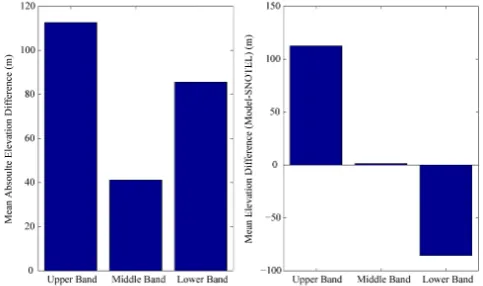
proximity. In order to show the representativeness of SNO-TEL stations in relation to the model elevation bands, Figs. 2 and 3 are presented. Figure 2 shows the vertical proximity of model elevation bands and their respective SNOTEL ob-servation site. It is important to note that model elevation bands above 2800 m and below 3400 m have relatively

28

Fig. 2. Scatter-plot comparing the elevation that each model band represents and the elevation of its respective SNOTEL observation site.

evidence that the middle elevation bands are well represented in terms of elevation in comparison to the low bias of obser-vations for the highest elevation bands and the high bias of the lowest elevation bands. Similar elevations between the model band and the SNOTEL observation are necessary for an accurate update because the timing of peak snowpack ac-cumulation changes dramatically with elevation. As will be described in the results, the elevation of the band also con-trols the timing of snowmelt, which strongly affects the mod-eling results. In order to account for the uncertainty in hor-izontal representativeness of the SNOTEL stations, which is strongly affected by the spatial distribution of forcing, vege-tation and wind, a temporally and spatially uncorrelated er-ror, with a standard deviation of 25 % of the observation, is considered for the SNOTEL SWE. This value was found to be adequate by examining the accuracy of the expected value and the reliability of probabilistic streamflow estimation dur-ing model hindcasts, usdur-ing Nash-Sutcliffe Efficiency, Rank Probability Skill Score and Normalized Root Mean Square Error for different error values. Of the error values explored, 25 % was found to produce the best verification scores on average, across all 15 study basins. In addition, uncorrelated errors were assumed for simplicity but the effects of corre-lated errors will need to be evaluated in future studies.

3 Experimental design

3.1 Data assimilation using the particle filter

The term data assimilation refers to a variety of techniques aimed at combining model simulation and observations to account for uncertainties in both state reconstruction tech-niques. In this study, ensemble based techniques are em-ployed because they directly address the prediction of un-certainty in the desired state. Of the available ensemble data assimilation techniques, the Ensemble Kalman Filter (EnKF) is the most popular in the hydrologic literature. Several

stud-29

Fig. 3. Mean absolute difference (left) and mean difference (right) between model elevation and its respective SNOTEL elevation. A positive mean difference indicates the model is at a higher elevation than its SNOTEL station.

ies in the past decade have applied this technique to hydro-logic models (Andreadis and Lettenmaier, 2006; Durand et al., 2009; Moradkhani et al., 2005a; Reichle et al., 2002; Roddell and Houser, 2004; Slater and Cark, 2006; Sun et al., 2004; Zaitchik and Rodell, 2009). Though these studies have shown that the EnKF is a valuable tool for data assimilation in many applications, this study focuses on the use of the Par-ticle Filter (PF). According to recent studies, the PF is an ef-fective hydrologic and hydraulics data assimilation method, providing predictive uncertainty in model states, parameters and fluxes (DeChant and Moradkhani, 2011a, b; Matgen et al., 2010; Leisenring and Moradkhani, 2010; Moradkhani et al., 2005b; Montzka et al., 2011; Rings et al., 2010; Weerts and El Serafy, 2006). The PF is not subject to the limitations experienced in the EnKF including the Gaussian assumption of joint distribution of observation and model states and the linear updating of model states (Moradkhani et al., 2005b; Moradkhani and Sorooshian, 2008). In addition, the PF is ca-pable of preserving the dynamical balance in the analysis (i.e. the conservation of mass) because the ensemble members are only resampled as opposed to being linearly adjusted, as in the EnKF (Moradkhani, 2008). Maintaining a water balance is assumed to beneficial in this framework, due to the water balance assumption in the SNOW-17, but the value of main-taining a water balance in a data assimilation framework has not been entirely quantified. For these reasons, the PF is used to assimilate the snow observations into the hydrologic mod-els.

In order to explain data assimilation, the modeling frame-work must be viewed in the state-space frameframe-work. The model is SNOW-17, which estimates the prior snowpack state based on the posterior snowpack states at the previous timestep and forcing data. As the model progresses forward in time, the prior distribution of states is produced according to Eq. (1).

x_i,t−=fx_i,t+₋₁,ui,t

+ωi,t (1)

where f is the forward operator (hydrologic model), x_i,t− represents the model predicted (prior) states (e.g. density, depth, liquid water in snowpack),x_i,t+₋₁ represents the up-dated model states at the previous time-step,ui,t represents the meteorological forcing data (precipitation and tempera-ture),ωi,t is the model error, which is normally distributed with a standard deviation of 25 % ofx_i,t−,i is the ensemble member and t is the time-step. This model error was termined in conjunction with SWE observation error as de-scribed in Sect. 2.3. Prior to update of the model states, an observational operator must be applied to transfer the states into the observation space, as in Eq. (2).

y_i,t0 =h

x_i,t−

+νi,t (2)

wherey_i,t0 is the prediction (SWE) andνi,t is the observation error.

Based on the recursive Bayes Law (3), the PF sequentially samples prior states and parameters to create an accurate pos-terior distribution, at each observation time-step.

p(xt|y1:t)=p(xt|yt,y1:t−1)=

p(yt|xt)p(xt|y1:t−1)

R

p(yt|xt)p(xt|y1:t−1)dx

(3) Equation (3) shows mathematically that a posterior condi-tional probability distribution of model predicted states (xt), given all previous observations (y1:t−1) and the current

ob-servation (yt), can be computed sequentially in time. The observation is the SNOTEL observed SWE. In this study, the probability of each particle, p(yt|xt), is calculated via the normal likelihood Eq. (4).

Lyt|xi,t−

=√ 1

2π√|Rk| exp

− 1

2Rk

yt−yi,t0 2

(4)

The normalized likelihood,p yt|xi,t,can easily be calcu-lated by:

pyt|x−i,t

=

Lyt|x−i,t

Np

P

i=1

Lyt|x_i,t−

=p yt−yi,t0 |Rk

(5)

In the above equations,Rkis the variance of the observations, which is 25 % as described in Sect. 2.3. This probability is necessary to transform the prior particle weights into the pos-terior via Eq. (6).

w+_i,t=

w_i,t−×pyt|xi,t−

Np

P

i=1

w−_i,t×pyt|xi,t−

(6)

In the PF with resampling, prior particle weights,w−_i,t, are set equal to 1/Np(Npis the number of particles) before moving

on to the next time-step. This results in a posterior weight,

w+_i,t,equal top yt|xi,twhich is the normalized likelihood. In this study, we rely on Sequential Importance Resampling (SIR) method as elaborated in Moradkhani et al. (2005b) and Moradkhani (2008). In the data assimilation portion of this study, 500 ensemble members, or “particles”, are used for snow estimation.

3.2 Ensemble streamflow prediction (ESP) with and without data assimilation

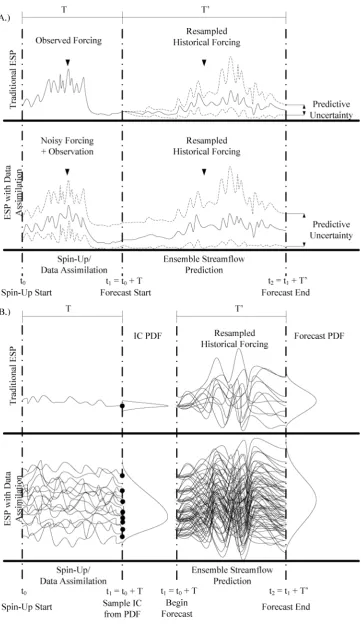
ESP is a method used by the NWSRFS to create probabilis-tic forecasts of seasonal streamflow volumes. This provides a prediction of the uncertainty in seasonal streamflow result-ing from unknown forcresult-ing data and initial model states at the time of forecast, as shown in Fig. 4. Initial model states are produced by running the model with observed input data up to the initial forecast time-step. This is called a “spin-up”. Starting at this point, the model is forced with resampled his-torical forcing, beginning at the initial forecast date, for each historical observation year. This produces a potential stream-flow trace that could occur given the current state of the land surface and a previously observed forcing dataset. Given that the assumptions of seasonal forcing stationarity and accurate model initial states are not violated, ESP can provide a skill-ful probabilistic prediction of seasonal streamflow.

ESP can be coupled with data assimilation for state initial-ization, also shown in Fig. 4. Rather than beginning the ESP forecast with a spin-up, as is done in traditional ESP, ESP-DA implements a data assimilation strategy to characterize the initial states. This creates an ensemble of state values that represent a probability density (Fig. 4b). After a sufficient number of time-steps, and assuming the uncertainty with re-spect to the model and observation are accurately quantified, the state distribution produced by data assimilation will ac-curately reflect the uncertainty in the state with respect to the model and observation. Similar to the spin-up, initialization through data assimilation requires many time-steps to reach reliable state values. At the forecast date, a given number of ensemble members are sampled from the state PDF, 50 in this study, and the ESP is performed from each of these en-semble members (shown in Fig. 4b with 8 sampled enen-semble members for visibility). This propagates the uncertainty from the initial condition through the ensemble forecast, which is hypothesized to create a more accurate estimation of uncer-tainty in streamflow prediction, as is represented in the fore-cast PDF in Fig. 4b.

30

Fig. 4. Diagram of the ESP and ESP-DA algorithms. (a) shows the uncertainty bounds of the data assimilation and forecast, (b) shows the individual traces generated from each sample.

Based on the reliability of ESP generated by sampling 50 ensemble members to different sample sizes, 50 ensemble members was found to balance the increase in computational demand, due to large sample size, and loss in reliability of the forecast, due to small sample size.

3.3 Performance metrics

Ranked Probability Score (RPS) is a widely used mea-sure for evaluating the quality of probabilistic predictions Wilks (2006). RPS is the sum of squared error of the cumu-lative probability forecasts averaged over multiple events. In streamflow prediction, the probability forecast is usually ex-pressed using a non-exceedance probability forecast within pre-specified categories (i.e. 1 %, 25 %, 50 %, 75 % and 99 % non-exceedance). The observed value for a given threshold (forecast category) takes on the value of 1 if the observed flow value is less than the threshold for that category. Oth-erwise, the observed value is 0. The discrete expression of RPS is given as:

RPSt= XJ

j=1

h

F_jt−O_jti

2

(7) where F_jt is the forecast probability at time t given by P(forecastj<threshj)and Ojt is the observed probability given by P(observed<threshj)wherej is the probability category. The Rank Probability Skill Score (RPSS) is also computed as the percentage improvement over a reference score (e.g. climatology) Wilks (2006):

RPSS= 1− RPS RPSref

!

×100= 1− RPS

RPSclimatology

!

×100 (8)

where RPSclimatologyis the rank probability score for the

ob-servation. A positive value shows to the percentage of im-provement over the reference RPS.

In the analysis of total streamflow volume, a rank his-togram and Q-Q plot are used to analyze the accuracy of the uncertainty prediction. In the Rank Histogram, the rank in which the observation falls on each ensemble prediction is presented. The rank is calculated according to the following equation.

Rankn=I yn,i0 < yn andyn,i0 +1> yn (9) wherey0 is the seasonal volumetric prediction andy is the observation, similar to the PF explanation. In addition, n is the index for each separate seasonal forecast. All ranks are then placed into a histogram. Since the ensemble vol-ume is assvol-umed to make up a probability density, a uniform histogram, in which the observation falls equally as often in each rank, indicates accurate representation of uncertainty. For a detailed description of Rank Histogram interpretation, see Hamill (2001) and Talagrand et al. (1997).

Similar to the rank histogram, a Q-Q plot provides infor-mation about the accuracy of the uncertainty estiinfor-mation of

the ensemble forecast. A Q-Q plot is created by first calcu-lating the normalized rank (z) of each observation

zn=

Iy_n,i0 < yn andyn,i0 +1> yn

N (10)

whereN is the total number of seasonal forecasts, which is 135 in this study. The ranks are then sorted and graphed. This graph is compared with a uniform line. A Q-Q plot matching the uniform line indicates a highly reliable forecast ensemble prediction. For details of the interpretation of a Q-Q plot, see Laio and Tamea (2007). While this plot is very useful in de-termining the effectiveness of the ensemble prediction, sup-portive quantitative scores are also included with this plot. Both the reliability and resolution, as described by Renard et al. (2010), can be adapted for this study to analyze the accuracy of probabilistic seasonal volume prediction. Equa-tions (12, 13 and 14) describe the two reliability statistics and Eq. (15) describes the resolution statistic.

α=1−2XN

n=1|zn−Un| (11)

ε=1−XN n=1

ε_n0

N (12)

ε0_n=

1 ifzn=1 orzn=0

otherwise 0 (13)

π= 1 N

XN n=1

E y_n0 SD[y0

n]

(14) With respect to the reliability of the forecast,αis a measure of the uniformity of the Q-Q plot (worst value is 0 and perfect score is 1) andεis a measure of the portion of observations inside the ensemble prediction (a value closer to 1 indicates a greater occurrence of observations falling within the ensem-ble). π is a measure of the resolution of the forecast, which will be referred to as precision. Given that two forecasts have similar reliability, the forecast with greater precision is pre-ferred because it indicates a lower level of uncertainty. In equation 12 through 15, U is the normalized uniform cu-mulative density. In equation 15,E[] is an expected value operator and SD[] is a standard deviation operator.

4 Results

31

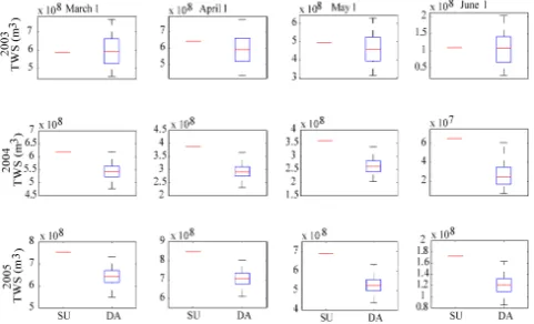
Fig. 5. Comparison of the total water stored (TWS) as snow pro-duced by the spin-up (SU) and data assimilation (DA) for the four forecast dates summed across all 15 basins.

the probability distribution of initial SWE values. The dis-tribution of snow states created by data assimilation repre-sents the uncertainty of the snow storage with respect to the model prediction and SNOTEL observations. From Fig. 5, it is observed that the spin-up and data assimilation display very different behavior through the three years. During 2003, the median TWS from data assimilation is near that of the model spin-up, but for the following two years there is a low bias for the data assimilation states, as compared to the spin-up model run. There are two factors creating this bias: the poor characterization of snowpack in the upper/lower eleva-tion bands by SNOTEL and the difference in yearly accumu-lation totals between the model and SNOTEL.

Poor representation of the upper and lower elevation bands by SNOTEL has important consequences on the accuracy of data assimilation. Since the observation is most representa-tive of the middle elevation band, the lowest elevation bands will be forced to peak later in the model than in reality, and the highest elevations will be forced to peak earlier in the model than in reality. Overall this causes a trend of miscal-culation of SWE in the winter months, when the majority of the flow would be from the lower elevation band, and late spring/summer months, when most of the flow would results from high elevation melt. Since SNOTEL is less representa-tive in the lower and upper elevation bands than the middle elevation band, it may be possible to improve the results by using different error characteristics for these bands. Though this would be a useful contribution to SNOTEL data assim-ilation in the Upper Colorado River Basin, this study does not attempt to manage these errors due to the complexity of melt timing differences between SNOTEL and the model. Because of the errors early and late in the snow accumula-tion/ablation season, the ESP-DA results are only expected to improve seasonal forecasts beginning on 1 March, 1 April and 1 May.

In addition to errors relating to the elevation of the obser-vations, the model and observations differ on the quantity of snow accumulation for each year. Figure 5 suggests that the model tends to produce similar snow quantities in each year while the SNOTEL stations have their greatest accumulation in 2003. This leads to a similar prediction of snow quantities in 2003 but a strongly low bias in the following two years. Though elevation differences between the model and SNO-TEL are expected to cause errors in the streamflow predic-tion, yearly differences are expected to improve the seasonal prediction. With an understanding of the effects that data as-similation has on model states during this time, the ensemble streamflow forecasts can be effectively analyzed.

Three month forecasts beginning in March and April are presented in Fig. 6 and beginning in May and June are pre-sented in Fig. 7. These figures show the cumulative runoff for each day in the forecast period, summed across all 15 study basins. Beginning in March, there is very little cumulative runoff through the first month. This is because the snow ac-cumulation will continue through most of March in a typical year. In April, an increasing amount of flow is observed, but it is not until May when the most rapid increase is ob-served. During May, most of the area within the 15 basins is experiencing significant snowmelt. These high flows do not taper off until late June. By late June, most of the snowpack has melted and only the highest elevations will have snow to melt. For most forecast dates, the uncertainty added through the initial states by data assimilation would be expected to increase the uncertainty in volumetric runoff. Rather than increasing the uncertainty, these figures suggest that the un-certainty is constrained by ESP-DA in comparison to ESP, through most forecasts. This is due to a generally low bias in the ESP-DA SWE in comparison to the ESP SWE. Since there is a lower boundary condition for the flow (baseflow), and no upper boundary condition, the low bias in the snow states has caused most of the ESP-DA forecasts to have less uncertainty in runoff volume than traditional ESP. During the 1 May and 1 June seasonal predictions for 2003, a larger uncertainty in initial conditions, with only a slight bias, is found to increase the seasonal volumetric prediction uncer-tainty. With respect to the 1 June prediction, it is important to note that, though the upper 95 % predictive bound of the ESP-DA is lower than that of the traditional ESP, the maxi-mum value of the ESP-DA is actually greater than that of the traditional ESP. This is shown by Fig. 8, which shows the to-tal 3 month volumetric streamflow forecast from all 15 basins for each forecast date. Overall for the forecasts beginning on 1 March, 1 April and 1 May, the biased predictions from ESP-DA, comparing to traditional ESP, appear to have more accurately bounded the observation. This is shown to im-prove the probabilistic prediction with an average imim-prove- ment in RPSS of 7.5 in 2004 and 11.5 in 2005. An improve-ment in RPSS suggests that the cumulative ensemble time series of prediction from ESP-DA is more accurate than tra-ditional ESP. Though an improvement was found in forecasts

32

Fig. 6. Cumulative daily volumetric flow plots summed across all 15 basins. This figure shows the 95 % predective bounds of the cu-mulative runoff volume from ESP (black lines) and ESP-DA (green lines). The expected value of each is a dashed line and the cumula-tive observed runoff volume is the red line.

33

Fig. 7. Similar to Fig. 6 but for 1 May and 1 June forecasts.

beginning March through May during 2004 and 2005, during other months ESP-DA performs worse than ESP. This result is consistent with the hypothesis that SNOTEL can only ac-curately constrain model snow prediction during the late win-ter and early spring months. As was discussed previously, the lack of representative observations of the lower and up-per elevation bands have led to poor snow estimation in the early and late ablation season. Since forecasts beginning in March, April and May are dominated by middle elevation band snowmelt, improved accuracy in middle elevation band snow has translated to more accurate flow predictions during these months. Though this analysis provides useful infor-mation about potential improvements that ESP-DA can have over ESP on a day by day forecast, it is arguably more impor-tant to look at the total seasonal volume, as this will likely be more useful information to reservoir management and water resources planning.

An analysis of the seasonal volume runoff prediction start-ing in March, April, May and June is provided in Fig. 8. This

34

Fig. 8. The volumetric flow summed across 15 basins for each sea-sonal forecast following the specific forecast dates. The dashed line indicates the observed value.

figure shows that the observed seasonal volume of flow from the 15 basins for all four seasonal forecasts starting between March and June falls within the ensemble prediction of both the ESP and ESP-DA. Though the total observed volume is within the predictive distribution from each method, the June prediction from ESP-DA has a clear low bias, which is not observed in the other three months. This is a result of the poor assimilation of upper elevation snow, which is the main source of runoff over the summer months. In general, Fig. 8 suggests that, in terms of total volume, the ESP and ESP-DA perform with similar accuracy for seasonal predictions beginning in March, April and May. Though the total vol-ume from all 15 study basins during the March, April and May seasonal predictions do not provide much evidence of an improvement in forecasting with ESP-DA, examining the volumetric flow predictions for each separate basin and start-ing date provides further information on the performance of ESP-DA.

35

Fig. 9. Rank histogram of the seasonal volumetric flow prediction for all 15 basins beginning in March, April and May during 2003, 2004 and 2005.

prediction with a slight low bias. In addition, the higherαfor ESP-DA, in relation to ESP, indicates a closer to uniform Q-Q plot, while a higherεindicates more observation lie within the ensemble range. This implies a generally more reliable prediction. It is also important to note that the ESP pro-duced a more precise prediction (as indicated by a largerπ value) than ESP-DA. This is expected because the ESP tech-nique accounts for fewer sources of uncertainty than ESP-DA. Overall the results suggest that seasonal predictions be-ginning in March, April and May in the upper Colorado River Basin more accurately characterize the uncertainty when ini-tialized by data assimilation than with a model spin-up.

5 Discussion and conclusion

This study examined the utility of incorporating ensemble data assimilation techniques to improve state initialization in the ESP framework by allowing for uncertainty in the ini-tial condition. A combined ESP-DA framework was im-plemented in 15 sub-basins in the upper Colorado River Basin. This was compared against traditional ESP to deter-mine if an improved representation of uncertainty could be achieved through data assimilation. Though positive results were found for ESP-DA, issues were found relating to the snow data assimilation.

In general, the flaws in this study stem from the lack of a representative observation for all basins. Since the SNOTEL stations tend to be in the range of middle elevation bands, the upper and lower elevation bands are known to be inaccu-rately adjusted. There is potential to improve the snow data assimilation in this study, either through more effective man-agement of errors relating to elevation misrepresentation, use of more realistic error assumptions (e.g. accounting for spa-tial and temporal error correlations), or use of more represen-tative datasets, but rigorous study is still needed in the field of snow data assimilation to achieve this. Though the

assim-36

Fig. 10. Q-Q plot of the seasonal volumetric flow predictions for all 15 basins beginning in March, April and May during the years 2003, 2004 and 2005.

ilation process is known to be flawed, some positive results can still be observed from this study. In the late spring and early summer, when the runoff is dominated by the middle elevation bands, the results presented here suggest that ESP can effectively be initialized through SNOTEL data assimi-lation. Furthermore, initialization through data assimilation can improve the ability to estimate seasonal runoff volume uncertainty. With this result, it can be inferred that as the understanding of snow data assimilation improves, ESP-DA will become more effective for seasonal streamflow predic-tion. This highlights the potential for accurate seasonal fore-casts in mountainous regions but emphasizes the need for im-proved snow estimation techniques to achieve a more accu-rate forecast.

In addition, the value of ensemble data assimilation within an operational framework is often debated. Ensemble data assimilation may become questionable in an operational framework due to the computational complexity. The NWS hydrologists currently implement run time modifications to adjust the state in model manually to improve forecasts. Manual adjustments require less computing time and it has yet to be proven that automatic data assimilation is more effective in state estimation than an experienced forecaster. One clear benefit of automatic data assimilation comes from an accurate accounting of initial condition uncertainty. Since data assimilation can characterize an entire initial condition PDF, not just initial condition adjustments, it is likely that au-tomated data assimilation will provide a more accurate char-acterization of uncertainty than manual modifications. In ad-dition, the computational demand may be a large obstacle for real-time forecasting at the NWS due to the daily time con-straints of the forecasts, but seasonal forecasting relaxes the time constraints on producing the forecast, therefore making ensemble data assimilation more attractive. For this reason, it is assumed in this paper that data assimilation is a viable technique for seasonal streamflow forecasting.

Overall this study found that ESP-DA has potential to im-prove characterization of uncertainty over ESP in snowmelt dominated basins. As expected, improvements were found during the period that achieved accurate state initialization. The results presented here show the importance of both ac-curate state initialization and acac-curate estimation of the un-certainty of the initial states. By more accurately charac-terizing the uncertainty in the states, the total seasonal flow uncertainty is more accurately represented. In future stud-ies, the ESP-DA techniques should be tested with new meth-ods for assimilating snow information and in different cli-matic regions to confirm the effectiveness of ESP-DA for different types of climates. ESP-DA can also be easily cou-pled with advanced techniques to constrain the forcing uncer-tainty. Therefore state initialization of ESP using data assim-ilation should be considered a potential tool for improving ESP forecasts in snow dominated basins.

Acknowledgements. Partial financial support for this research was

provided by NOAA-CPPA, Grant No. NA07OAR4310203. We are grateful to NWS-CBRFC for providing us with some of the data used in this study. We would also like to thank Mohammad Reza Najafi for his early contribution to the ESP setup of this experiment. In addition, we thank the four reviewers for useful comments on improving this manuscript.

Edited by: A. Weerts

References

Anderson, E. A.: National Weather Service river forecast system-snow accumulation and ablation model, TECHNICAL MEMO-RANDUM NWS HYDRO-17, November 1973, 217 pp., 1973. Andreadis, K. M. and Lettenmaier, D. P.: Assimilating

remotely sensed snow observations into a macroscale hydrology model, Adv. Water Resour., 29, 872–886, doi:10.1016/j.advwatres.2005.08.004, 2006.

Burnash, R. J. C., Ferral, R. L., and McGuire, R. A.: A generalized streamflow simulation system: Conceptual modeling for digital computers, US Dept. of Commerce, National Weather Service, 1973.

Day, G. N.: Extended streamflow forecasting using NWSRFS, J. Water Res. Pl.-ASCE, 111, 157–170, 1985.

DeChant, C. and Moradkhani, H.: Radiance data assimilation for operational snow and streamflow forecasting, Adv. Wa-ter Resour., 34, 351–364, doi:10.1016/j.advwatres.2010.12.009, 2011a.

DeChant, C. and Moradkhani, H.: Examining the Effectiveness and Robustness of Sequential Data Assimilation Methods for Quan-tification of Uncertainty in Hydrologic Forecasting, Water Re-sour. Res, in review, 2011b.

Durand, M., Kim, E. J., and Margulis, S. A.: Radiance assimi-lation shows promise for snowpack characterization, Geophys. Res. Lett., 36, L02503, doi:10.1029/2008GL035214, 2009. Hamill, T. M.: Interpretation of rank histograms for

verify-ing ensemble forecasts, Mon. Weather Rev., 129, 550–560, doi:10.1175/1520-0493(2001)129¡0550:IORHFV¿2.0.CO;2, 2001.

Kennedy, A. M., Garen, D. C., and Koch, R. W.: The association between climate teleconnection indices and Upper Klamath sea-sonal streamflow: Trans-Nino Index, Hydrol. Process., 23, 973– 984, doi:10.1002/hyp.7200, 2009.

Laio, F. and Tamea, S.: Verification tools for probabilistic forecasts of continuous hydrological variables, Hydrol. Earth Syst. Sci., 11, 1267–1277, doi:10.5194/hess-11-1267-2007, 2007. Leisenring, M. and Moradkhani, H.: Snow Water Equivalent

Esti-mation using Bayesian Data Assimilation Methods, Stoch. Env. Res. Risk A., 25, 253–270, doi:10.1007/s00477-010-0445-5, 2010.

Li, H., Luo, L., Wood, E. F., and Schaake, J.: The role of initial conditions and forcing uncertainties in sea-sonal hydrologic forecasting, J. Geophys. Res., 114, D04114, doi:10.1029/2008JD010969, 2009.

Lorenz, E. N.: Climate predictability, the physical basis of climate and climate modeling, WMO GARP Publication Series, 16, 132– 136, 1975.

Matgen, P., Montanari, M., Hostache, R., Pfister, L., Hoffmann, L., Plaza, D., Pauwels, V. R. N., De Lannoy, G. J. M., De Keyser, R., and Savenije, H. H. G.: Towards the sequential assimilation of SAR-derived water stages into hydraulic models using the Par-ticle Filter: proof of concept, Hydrol. Earth Syst. Sci., 14, 1773– 1785, doi:10.5194/hess-14-1773-2010, 2010.

McGuire, M., Wood, A. W., Hamlet, A. F., and Lettenmaier, D. P.: Use of satellite data for streamflow and reservoir storage fore-casts in the Snake River Basin, J. Water Res. Pl.-ASCE, 132, 14 pp., doi:10.1061/(ASCE)0733-9496(2006)132:2(97), 2006. Montzka, C., Moradkhani, H., Weihermuller, L., Canty, M.,

Hendricks Franssen, H. J., Vereecken, H.: Hydraulic Param-eter Estimation by Remotely-sensed top Soil Moisture Ob-servations with the Particle Filter, J. Hydrol., 399, 410–421, doi:10.1016/j.jhydrol.2011.01.020, 2011.

Moradkhani, H.: Hydrologic Remote Sensing and Land Surface Data Assimilation, Sensors, 8, 2986–3004, doi:10.3390/s8052986, 2008.

Moradkhani, H. and Meier, M.: Long-Lead Water Supply Forecast Using Large-Scale Climate Predictors and Inde-pendent Component Analysis, J. Hydrol. Eng., 15, 744, doi:10.1061/(ASCE)HE.1943-5584.0000246, 2010.

Moradkhani, H. and Sorooshian, S.: General review of rainfall-runoff modeling: Model calibration, data assimilation, and un-certainty analysis, Hydrological Modeling and the Water Cycle, 63, doi:10.1007/978-3-540-77843-1 1, 2008.

Moradkhani, H., Sorooshian, S., Gupta, H. V., and Houser, P. R.: Dual state-parameter estimation of hydrological models us-ing ensemble Kalman filter, Adv. Water Res., 28, 135–147, doi:10.1016/j.advwatres.2004.09.002, 2005a.

Moradkhani, H., Hsu, K. L., Gupta, H., and Sorooshian, S.: Un-certainty assessment of hydrologic model states and parameters: Sequential data assimilation using the particle filter, Water Re-sour. Res., 41, W05012, doi:10.1029/2004WR003604, 2005b. Moradkhani, H., Hsu, K., Hong Y., and Sorooshian, S.:

Investigat-ing the Impact of Remotely Sensed Precipitation and Hydrologic Model Uncertainties on the Ensemble Streamflow Forecasting, Geophys. Res. Lett., 33, L12401, doi:10.1029/2006GL026855, 2006.

Forecast System Reanalysis, J. Hydrol., in review, 2011. Pagano, T., Garen, D., and Sorooshian, S.: Evaluation of

official western US seasonal water supply outlooks, 1922– 2002, J. Hydrometeorol., 5, 896–909, doi:10.1175/1525-7541(2004)005¡0896:EOOWUS¿2.0.CO;2, 2004.

Regonda, S. K., Rajagopalan, B., Clark, M., and Zagona, E.: A multimodel ensemble forecast framework: Application to spring seasonal flows in the Gunnison River Basin, Water Resour. Res., 42, 9404, doi:10.1029/2005WR004653, 2006.

Reichle, R. H., McLaughlin, D. B., and Entekhabi, D.: Hy-drologic data assimilation with the ensemble Kalman filter, Monthly Weather Review, 130, 103–114, doi:10.1175/1520-0493(2002)130¡0103:HDAWTE¿2.0.CO;2, 2002.

Renard, B., Kavetski, D., Kuczera, G., Thyer, M., and Franks, S. W.: Understanding predictive uncertainty in hydrologic mod-eling: The challenge of identifying input and structural errors, Water Resour. Res., 46, W05521, doi:10.1029/2009WR008328, 2010.

Rings, J., Huisman, J. A., and Vereecken, H.: Coupled hydrogeo-physical parameter estimation using a sequential Bayesian ap-proach, Hydrol. Earth Syst. Sci., 14, 545–556, doi:10.5194/hess-14-545-2010, 2010.

Rodell, M. and Houser, P. R.: Updating a land surface model with MODIS-derived snow cover, J. Hydrometeorol., 5, 1064–1075, doi:10.1175/JHM-395.1, 2004.

Slater, A. G. and Clark, M. P.: Snow data assimilation via an ensemble Kalman filter, J. Hydrometeorol., 7, 478–493, doi:10.1175/JHM505.1, 2006.

Sun, C., Walker, J. P., and Houser, P. R.: A methodology for snow data assimilation in a land surface model, J. Geophys. Res., 109, D08108, doi:10.1029/2003JD003765, 2004.

Talagrand, O., Vautard, R., and Strauss, B.: Evaluation of proba-bilistic prediction systems, paper presented at ECMWF Work-shop on Predictability, Eur. Cent. for Med. Range Weather Fore-casts, Reading, UK, 1997.

Tang, Q. and Lettenmaier, D. P.: Use of satellite snow-cover data for streamflow prediction in the Feather River Basin, California, Int. J. Remote Sens., 31, 3745–3762, doi:10.1080/01431161.2010.483493, 2010

Thirel, G., Rousset-Regimbeau, F., Martin, E., and Habets, F.: On the impact of short-range meteorological forecasts for ensem-ble streamflow predictions, J. Hydrometeorol., 9, 1301–1317, doi:10.1175/2008JHM959.1, 2008.

Twedt, T. M., Schaake Jr., J. C., and Peck, E. L.: National Weather Service extended streamflow prediction, in: Proc. 45th Western Snow Conference, Albuquerque, NM, Colorado State University, 52–57, 1977.

Weerts, A. H. and El Serafy, G. Y. H.: Particle filtering and ensem-ble Kalman filtering for state updating with hydrological con-ceptual rainfall-runoff models, Water Resour. Res., 42, W09403, doi:10.1029/2005WR004093, 2006.

Wilks, D. S.: Statistical methods in the atmospheric sciences, (In-ternational geophysics series), 2006.

Wood, A. W. and Lettenmaier, D. P.: An ensemble approach for attribution of hydrologic prediction uncertainty, Geophys. Res. Lett., 35, L14401, doi:10.1029/2008GL034648, 2008.

Zaitchik, B. F. and Rodell, M.: Forward-Looking Assimilation of MODIS-Derived Snow-Covered Area into a Land Surface Model, J. Hydrometeorol., 10, 130–148, 2009.