Deformation Behavior and Mechanical Analysis of Vertically Aligned Carbon Nanotube (VACNT) Bundles

(1)

ANALYSIS OF VERTICALLY ALIGNED CARBON

NANOTUBE (VACNT) BUNDLES

Thesis by

Shelby B. Hutchens

In Partial Fulfillment of the Requirements for the Degree of

Doctor of Philosophy

California Institute of Technology Pasadena, California

2011

(2)

(3)

Acknowledgements

I have had a rich and defining experience during my period at Caltech. Though many times I did not take the smoothest or most efficient path, I am very thankful to have had to opportunity to make the mistakes and overcome the obstacles that are now a cherished part of who I am as a researcher and an individual. Many people have assisted me with guidance, empathy, wisdom, and distraction when needed. I would like to thank a few especially.

The two people most responsible for my progression as a researcher are my advisors, Professors Zhen-Gang Wang and Julia R. Greer. Professor Wang consistently provided me with clear, neutral, and unaffected advice. Through his guidance I learned what it means to think deeply about scientific problems and address them with rigor, though I did not always appreciate this lesson as it was being taught. I am very grateful to have had the opportunity to know and work with him. Professor Greer has provided me with a shining example of the kind of person, science and otherwise, that I would like to become. She and her group also reintroduced me to the excitement and fun of science. I am eternally grateful for every chance she gave me to participate in the scientific community as a part of conferences, workshops, and meetings. These experiences, with her example to guide me, have helped to give me both the perspective and confidence I lacked and continue to improve upon. I also appreciate all of the time she so generously gave me in one-on-one conversations. Her insight has provided me with lessons that have shaped the way that I see the world around me, particularly science questions and my interactions with others.

I would also like to express my appreciation to our collaborator, Professor Alan Needle-man, for his time, frank input, wisdom, and patience. Thanks to Professor Greer, I have been truly lucky to have had the chance to interact so closely with him.

(4)

freely given confidence and friendship. She is an inspiration both scientifically and as a human being. I look forward to our lifelong friendship and am thankful to have met her. I am grateful for the friendship and support of my fellow incoming class of chemical engi-neering women and the “girly” lunches we shared: Heather Hunt, Lisa Hochrein, Arwen Brown, and Heather McCaig. I am indebted to all of the members of the Greer group, particularly Andrew Jennings and Dongchan Jang, from whom I learned my appreciation of scientific discussion and debate. I wish to express my gratitude to the Danger Twins and company for welcoming me without judgement, to every visiting speaker I hosted for the advice they so willingly gave, and to all of my summer students for the opportunity to learn through our interactions. I would also like to recognize Josh Spurgeon; our time together is a treasured memory.

Finally, I would like to thank my family, whose support of and faith in my ability got me to a position where I could reap all of the benefits of the aforementioned relationships. A thank you goes in particular to my mother, I love you very much, and I one day hope to attain your level of optimism.

I think my graduate experience can best be summed up by an adage I received in a recent email from Professor Needleman.

I may have told you about experience:

How did you learn how to make good decisions? Experience. How did you get experience? Bad decisions.

(5)

Abstract

(6)

(7)

Bibliography 110 A Testworks Compression Method 114 B Testworks Compression Method 118 C FIB Procedure for VACNT pillar 121 D Simulated CNT Images 123 E Free Energy Expressions for Differing Dielectric Constants 124 F Toward a DFT Approach to Polyelectrolyte Behavior in Small Systems 125 F.1 Introduction . . . 125

F.2 Theoretical Framework . . . 125

F.3 Osmotic Pressure for Small Systems . . . 130

F.3.1 Derivation of Osmotic Pressure . . . 130

(10)

List of Figures

1.1 Carbon nanotubes . . . 2

1.2 Vertically aligned carbon nanotubes. . . 3

1.3 Typical foam stress-strain response . . . 5

2.1 VACNT cylindrical pillar samples . . . 10

2.2 FIB milled pillar . . . 11

2.3 Ion milled flat punch indenter tip for microcompressions . . . 13

2.4 Ion milled flat punch indenter tip forin situmicrocompressions . . . 13

2.5 Schematic of the Agilent Nanoindenter G200 XP head . . . 14

2.6 Simple harmonic oscillator model of the Agilent Nanoindenter G200 XP head 15 2.7 Fit of XP head to simple harmonic oscillator model . . . 16

2.8 Indenter head mass . . . 17

2.9 Machine stiffness as a function of raw displacement . . . 18

2.10 Machine damping as a function of raw displacement . . . 18

2.11 Determination of cutoff frequency . . . 19

2.12 Viscoelastic model of the Agilent G200 Nanoindenter XP system . . . 22

2.13 Applied displacements for constant strain rate tests of VACNT micropillars . 24 2.14 Schematic of thein situtesting setup . . . 28

2.15 Photo of thein situtesting instrument, SEMentor . . . 29

3.1 Illustration of the apparent axial tube number density gradient . . . 31

3.2 TEM images of the multiwall CNTs making up the VACNT bundles . . . 32

3.3 Image series illustrating tube density gradient . . . 33

3.4 Characteristics of typical experimental and simulated CNT images . . . 35

(11)

3.6 Power spectra quantification of simulated microstructure images . . . 39

3.7 Gaussian bandpass filtered CNT micrographs. . . 40

4.1 Stress-strain responses from CNT micropillar compressions . . . 49

4.2 Post-mortem CNT pillars . . . 50

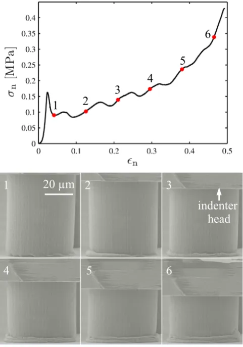
4.3 In situillustration of bottom - to - top sequential periodic buckling . . . 50

4.4 In situvideo of uniaxial microcompression (electronic version only) . . . 51

4.5 In situillustration of buckle nucleation and propagation . . . 52

4.6 In situmicrographs of initial sudden collapse event . . . 53

4.7 In situvideo of several initial buckling events (electronic version only) . . . . 54

4.8 High magnification SEM images of a deformed VACNT micropillar . . . 55

4.9 Viscoelastic characterization of VACNT micropillars . . . 57

4.10 Normalized storage and loss stiffness . . . 58

5.1 Summary ofin situresults . . . 61

5.2 Plastic hardening function . . . 64

5.3 Comparison of simulated and experimental results . . . 67

5.4 Deformed meshes and contour plots . . . 69

5.5 Effect of flow strength parameters on buckle formation . . . 70

5.6 Effect of flow strength parameters on buckle wavelength and magnitude . . . 73

5.7 Influence of a strength gradient on the model results . . . 77

7.1 Charged cluster in an ion solution . . . 91

7.2 Size dependence of the free energy of electrostatic interaction . . . 94

7.3 Electrostatic potential profiles . . . 99

7.4 Free energy of cluster formation . . . 104

7.5 Phase diagram for a unimer . . . 105

7.6 Cluster density profiles . . . 106

7.7 Micelle-like behavior of charged cluster formation . . . 107

A.1 Testworks compression method overview . . . 116

(12)

(13)

List of Notation

Following is a list of mathematical symbols used in this thesis. Only symbols used through-out the thesis are presented. The page on which the symbol is first defined is given on the right.

˙ indicates the time derivative of a variable . . . 63

n nominal or engineering strain . . . 48

t true strain . . . 67

ν Poisson’s ratio . . . 26

σn nominal or engineering stress . . . 48

σt true stress . . . 74

φ phase angle . . . 15

E Young’s or elastic modulus . . . 23

f frequency, in Hz . . . 15

H pillar height before deformation . . . 48

ph harmonic load amplitude . . . 15

R pillar radius before deformation . . . 48

uh harmonic displacement amplitude . . . 15

(14)

Chapter 1 Introduction

The study of materials science is typified by the relationships between a material’s struc-ture, properties, and processing. Characterization of these relationships yields a full de-scription of the material of interest. This thesis focuses largely on the first two aspects, structure and properties, for a structure composed of vertically aligned carbon nanotubes (VACNTs) while bearing in mind the influence of processing on the samples tested and the information reported in the literature. VACNTs can be grown in macroscopic, continuous films and have become materials of interest due to both their relative ease of growth with respect to other fullerene-based structures and the unique properties of their carbon nan-otube building blocks. In addition, they have shown promise in a wide array of applications many of which take advantage of their inherently multifunctional nature. The focus in the following study has been on the mechanical response of these materials, particularly under compression, in which they show an unusual structural response that is explored through

in situ experiments and finite element analysis. These observations of VACNT structure and microstructure lead to increased understanding of the mechanisms responsible for and constitutive stress-strain relationship of their complex, local material behavior.

1.1 Definition and General Characteristics of Vertically

Aligned Carbon Nanotubes

(15)

struts. Promising thermal, electrical, and mechanical properties have made carbon nan-otubes (CNTs) the subject of study in fields ranging from medicine to electronics [1–4]. A single walled CNT (SWCNT) generally has a diameter close to 1 nm and is composed of a single sheet of graphene, a monolayer of carbon atoms in a hexagonal arrangement, in the shape of a cylinder (see Fig. 1.1(a)). Multiwalled carbon nanotubes (MWCNTs) consist of multiple concentric layers of graphene-like sheets ranging from two (double-walled CNTs) to several, with a sheet to sheet spacing of 3.4 ˚A[5] and diameters typically less than 100 nm [6]. Experiments have demonstrated thermal conductivities on the order of 200 W m−1 K−1for bulk single-walled CNTs and 3000 W m−1K−1for an individual MWCNT [7] with theoretical predictions for the single-walled tube as high as 2980 W m−1 K−1 [8]. These numbers are 10 times those of conventional materials, i.e., metals. CNTs are also unique in that they can display both metallic and semiconducting electrical properties depending on their chirality (Fig. 1.1(a)). In their metallic configuration, they have a high electrical conductivity, comparable to that of Cu [9]. Most relevant to this work, MWCNTs have been shown to be one of the strongest materials tested, having a tensile modulus on the

armchair zig-zag helical

0.36 nm

0.34 nm

a)

b)

[image:15.595.111.469.453.661.2]

c)

(16)

order of 1 TPa and a strength of tens of GPa [9]. However, due to their high aspect ratio (length/radius), MWCNTs bend or buckle readily when subject to compressive loads, do-ing so at much lower loads than those required for yield in tension. They have been shown to bend as much as 120◦ without breaking atomic bonds [10], enabling them to recover almost completely after such deformation. It is for all of these features that CNTs are a vast and prominent area of study. When combined to create a VACNT material they form a complex, hierarchical structure that bridges the gap between the nano and macro scales while maintaining many of the promising mechanical, thermal, and electrical properties of individual tubes and displaying new aspects of each arising from the collective interactions of the tubes.

Generally, VACNTs are nominally vertically aligned arrays of carbon nanotubes grown perpendicularly from a stiff substrate, typically Si or Quartz. The term vertically aligned carbon nanotubes comes from the fact that at relatively low magnifications, 1000×, the tubes appear highly aligned as illustrated in Fig. 1.2. It is because of this that they have also been referred to as CNT turfs, forests, brushes, mats, and foams. At 100× higher magnifications (center image in Fig. 1.2), the CNTs are found to be intertwined with and adhered to each other. At this lengthscale, the anisotropy that was so obvious at lower magnification now begins to disappear in favor of isotropy. Magnifying 100×more (right image in Fig. 1.2), the transmission electron microscopy (TEM) image individual structure

10 μm 200 nm 10 nm

Anisotropic

aligned tubes foam-like network

Isotropic

individual tube

Discrete

(17)

of the MWCNTs. This specific geometry differs from shorter forests in which tubes are either less tightly packed or shorter, preventing in complex tube entanglement that is one of the defining characteristics of VACNTs. The microstructure is also unlike CNT conglom-erates or CNT composite materials in that there is typically no anisotropy due to nominal alignment in either of these examples.

VACNTs are relatively easy to grow and pattern. A typical synthesis technique is that of chemical vapor deposition (CVD) at atmospheric pressure and temperatures around 750 ◦

C [11]. A precursor gas (e.g., ethylene) is flowed across a thin layer of catalyst (e.g., Fe) supported by a wafer substrate (e.g., Si or quartz). There are many issues with and studies on the growth mechanisms of VACNTs including efforts to control density, alignment, tube diameter, wall number, and chirality [12] that are beyond the scope of this thesis. Using the CVD technique, samples nearly 2 cm tall have been grown [6]. Typically the tubes in these materials are MWCNTs, as high purity SWCNTs are more difficult to obtain. Creation of a continuous film versus a patterned VACNT structure is often achieved through selective catalyst deposition, with photolithographic patterning of the catalyst leading to patterned VACNTs. Alternative growth techniques include simultaneous flow of both the precursor gas and the catalyst during CVD [13] and high temperature vacuum decomposition [14], which only results in very short arrays of less than 1µm tall, to mention a few. The specifics of the growth process utilized for this thesis, based on the typical CVD techniques discussed first, are given in detail in Section 2.2.1.1.

1.2 Applications

(18)

thermally robust energy dissipating rubber [14, 19, 20], and energy absorption or impact mitigation [13, 21, 22]. Even in applications where the mechanical behavior is not central to design or implementation, an understanding of the mechanisms of deformation and fa-tigue behavior is essential for analysis of the life-in-use of the device. Several properties unique to VACNTs make them desirable candidates for these applications. First, VACNTs are unique in that they are both soft materials, due to the reduced load capacity of the CNT struts as they bend, and highly conductive materials, both electrically and thermally, while being thermally robust and non-oxidizing. Thermal contacts for MEMS and other micro-electronic systems look to take advantage of their simultaneous thermal conductivity, or ability as a heat sink, and their compliance, in order to avoid damaging delicate features. Additionally, VACNT’s hierarchical structure allows them to conformally contact surfaces, which is necessary both in maximizing thermal transfer and for increasing bonding between surfaces in the case of dry adhesives. In the case of dry adhesives, also called CNT tapes, the large contact area combined with the properties of the tubes themselves enable the ma-terial to withstand shear stresses of 36 N/cm2, nearly four times higher than the gecko foot, as well as to stick to a variety of surfaces, including Teflon [17].

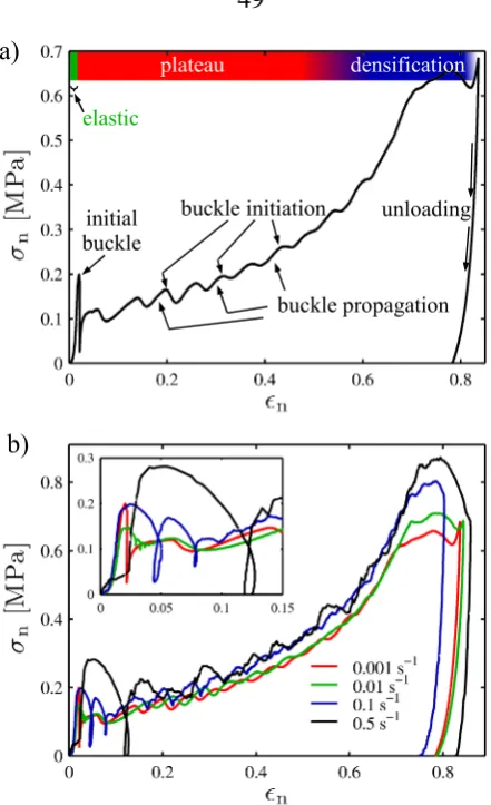
The interconnected, network-like structure of VACNTs closely resembles foams or other fibrous structures which traditionally find use as energy absorbers. In this application, the CNTs serve as the struts supporting the open structure of the material. A stress-strain curve for a characteristic elastic-plastic foam is shown in Figure 1.3. This response

(19)

cludes three distinct regimes: elastic loading, a stress plateau, and densification. The open structure allows for accommodation of large deformation for minimal changes in applied load throughout the plateau regime during which the struts bend and buckle. The result is a large area under the stress-strain curve that translates to a large amount of energy absorbed. When viewed in this framework, the CNTs, connected through their intertube interactions, serve as the struts supporting the open structure of the material. By nature, these struts are both strong and lightweight, making them ideal candidates. In fact, VACNTs have been ob-served to undergo an overall foam-like response [24], but do so in a highly localized manner that is very different from traditional foams as will be discussed in detail in Chapter 4.

Additionally, experiments have shown VACNTs to exhibit highly viscoelastic behavior. Researchers have surmised that energy dissipation in these materials arises from sliding and reorganization between tubes [19, 20] though detailed studies of the mechanism have not been reported at the time of this writing. This viscoelastic response, combined with their thermal robustness, enables VACNTs to act as energy dissipators or dampers at tempera-tures where traditional damping materials, i.e., polymers, become brittle (low temperatempera-tures) or ineffective (high temperatures).

1.3 Objectives and Scope

The objective of this thesis is to explore the mechanical deformation behavior of a class of materials known as vertically aligned carbon nanotubes. Specifically, the focus is on a rela-tively new, unusual, and largely unstudied phenomenon recently observed in VACNTs, that of sequential periodic buckling in VACNTs under uniaxial loading. This rich mechanical behavior is characterizedin situand used to motivate a constitutive relation for these com-plex, multiscale materials that may one day be utilized for capturing the structural response of these materials in any geometry.

(20)

(21)

Chapter 2 Experimental Procedure

2.1 Introduction

Mechanical properties are extracted from materials in a wide variety of methods including notched fracture testing, nanoindentation, bending tests, tension, plane strain or stress, and the list goes on. In this thesis, uniaxial compression tests are the chosen testing method for several reasons. First, nanoindentation, while simple in setup because it requires little specialized sample preparation and therefore can be performed quickly, is difficult to an-alyze. Stress concentrations occur at the indenter’s tip or its edge (depending on indenter geometry) and corresponding strain gradients can make characterization of non-elastic or non-monolithic materials behavior non-trivial, particularly when deformation mechanisms are poorly understood as with VACNTs. Additionally, geometry independent mechanical variables like stress and strain are difficult or impossible to calculate. Second, energy ab-sorption and dissipation applications motivate this work. Since these applications would utilize VACNTs in compression, fracture, bending, and tension tests are less applicable. Plus, uniaxial compressions enable straightforward analysis in terms of engineering stress and strain, as will be discussed in Section 2.4. Finally, experiments are performed on small scale samples via microcompression (in a nanoindenter) as opposed to macrocompressions in order to resolve load–displacement features occuring at low loads as well as conduct

(22)

In order to extract the sample’s load–displacement response from the raw load and displacement data gathered during an experiment, the complete description and characteri-zation of the indenter system must be obtained. This description and procedure is described in Section 2.3. A model of the indenter-plus-sample system is discussed in Section 2.4in order to correctly deconvolute the sample and testing system responses. In Section 2.5 a method for dynamic mechanical analysis that allows the viscoelastic response of a material can be characterized is described. This method measures the storage and loss stiffnesses of a material, which can be functions of the frequency of excitation. Finally, a description of thein situmicromechanical testing setup, SEMentor, is given in Section 2.6.

2.2 Sample and Nanoindenter Tip Fabrication for

Uniax-ial Testing

In order to obtain the desired uniaxial testing geometry specialized sample geometries, circular cylinders, as well as two flat punch nanoindenter tips forin situand ex situ testing are produced.

2.2.1 VACNT sample preparation

Cylindrical samples of VACNTs, which will be referred to interchangeably as both pillars and bundles, were created using the two methods described below. Cylindrical samples were initially prepared using a focused ion beam (FIB) to mill CNT material out of a continuous CNT film. Poor sample quality with this method lead to acquiring prepatterned cylindrical samples through a collaboration with Lee J. Hall and Harish Manohara at the Jet Propulsion laboratory.

2.2.1.1 Photolithographically patterned VACNT pillars

Pillars of VACNTs, also called CNT bundles, are grown on a generic Si wafer (with∼ 300-–400 nm thermal oxide) patterned using contact photolithography, then cleaned with O2

(23)

chamber is vented to atmosphere to allow the Al to oxidize, forming an Al2O3barrier layer.

This layer performs the function of reducing diffusion of the Fe catalyst into the substrate which can interfere with CNT growth. Next, a∼2.5–3.0 nm layer of active catalyst Fe is evaporated. The lift-off process removes the photoresist leaving only the patterned catalyst, and the wafer is placed in a 2 inch diameter quartz tube, single zone furnace outfitted with vacuum exhaust and an automated throttle valve. The quartz tube is purged and filled with Ar (99.999% pure Ar, ‘UHP’ grade from Airgas) 3 times, then pressure is held at 200 Torr while flowing Ar at 500 sccm and simultaneously ramping the temperature to 675 ◦

C. When the temperature is stable at 675◦C, Ar is quickly switched out and a flow of 500 sccm of ethylene (99.995% C2H4, ‘Research Grade’ from Airgas) is begun in order to grow

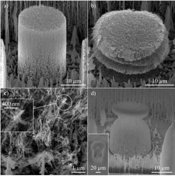
the multiwall CNTs. Run times are typically between 15 and 30 minutes. To end growth, the Ar and ethylene are quickly switched again and the furnace is allowed to cool to near room temp under flowing Ar. This method is discussed in further depth in Manohara et. al. [25] and references therein. These samples, whose mechanical deformation is described in this thesis, were grown by Lee J. Hall at the Jet Propulsion Laboratory. Samples are chosen from the array of grown pillars using an SEM according to three criteria: They adhere to the desired cylindrical shape (no missing parts, few stray tubes), they are perpendicular to the substrate (see Fig. 2.1), and their aspect ratio is between 1 and 1.5.

10 m 50 m

a) b)

(24)

2.2.1.2 Focused Ion Beam Milled VACNT pillars

VACNTs are most easily and more commonly grown in continuous films. Therefore, it is of some interest to develop a method for small scale testing of the properties of these continuous films in uniaxial compression. Following methods utilized for creating uniaxial compression samples for small scale metallic samples, annuli were milled in the VACNT material, resulting in pillars. The continuous, VACNT films were grown via CVD and obtained through a collaboration with Chiara Daraio of Caltech. The milling was done under the focused ion beam (FIB) of a dual beam system (FEI Nova 200). FIB milling

10 m

10 m 10 m

20 m

a) b)

d)

1 m 400 nm

[image:24.595.143.504.292.657.2]

c)

(25)

was enhanced through the use of the selective carbon mill, which is essentially a needle that injects water vapor close to the area being milled in order to increase the oxidation of carbonaceous materials into CO2 [26]. The milling was performed at a series of ion beam

currents starting at 7 nA for removal of large regions of material and gradually decreasing to 3 nA for cleaner results toward the end. Sample geometries created typically had a radius of 20µm or 50µm with an aspect ratio (height/radius) of 2.5. Images of the pre- and post-compression FIB milled pillars illustrate the results achieved with this process (Figs. 2.2(a) and (b)). The milling process was prone to the accumulation of redeposition in the milled region around the pillar and on the outer edge of the pillar itself (see Figure 2.2). Attempts were made to minimize these anomalies by careful milling in sequentially smaller annuli, but their reduction to an acceptable level was never realized. An attempt to remove the redeposition was made using an oxygen plasma etcher. Unfortunately, this treatment results in removal of the VACNTs themselves, a deformed pre-compression pillar, and almost no removal of the redeposition (Fig. 2.2(d)). Post-compression images of FIB milled microcompression samples showed fracture in the difficult to remove redeposition (Fig. 2.2(c)). Additionally, the pillar and the flat punch interact with the remaining redeposition structures that surround it, as evidenced by the inset in Fig. 2.2(c). Thus, the mechanical response of the VACNT material was certainly convoluted with the mechanical response of the FIB redeposition and this sample preparation method was deemed unacceptable. The milling schedule for a 50µm diameter pillar is given in Appendix C.

2.2.1.3 Diamond Indenter Tip Fabrication

(26)

punch (Fig. 2.3) took over 550 hours to mill at 20 nA current and was designed to be mounted in the G200 system. The final geometry has a diameter of approximately 100µm and a length of approximately 90 µm. The smaller, rectangular flat punch (Fig. 2.4) has a width of 80 µm and a depth of 60µm with a miniature flat punch (effectively 5 µm ×

5µm) attached to the side for compression of smaller bundles of CNTs. Its height is only 30 µm because displacement in the SEMentor is limited to 30µm so any further height increase is unusable.

100 m 50 m

Figure 2.3: Top (left) and side (right) views of the diamond flat punch indenter tip after focused ion beam milling from a Berkovitch tip geometry.

20 m

(27)

2.3 Characterization of Micromechanical Testing System

An understanding of the testing instrumentation is a necessary precursor to performing ex-periments, as knowledge of the measurement limitations guides experimental design and enables proper data collection. Compression tests were mostly carried out in an Agilent Nanoindenter G200 system using the XP head (comes from ‘explorer’). The XP head was used as opposed to the DCM (dynamic contact module), which is also available on the testing instrument. While the DCM head is characterized by superior load resolution and displacement control, because the DCM it is limited to a maximum travel distance of 30µm (and is really only intended for half of that) full compression of the samples is impossible and it is not used in testing. The XP head essentially consists of a electromagnetic load-ing cell, loadload-ing column, leaf sprload-ings, capacitive displacement gauge, and indenter tip all mounted within a stiff loading frame. A schematic of the relationship between these parts is shown in Figure 2.5. The leaf springs support the column while load is applied through the inductive coil/magnet assembly, making the system inherently load controlled. Dis-placement is measured via the capacitor with a zero raw disDis-placement,uraw, position being

defined at the center of the capacitive range. Raw displacement can vary between −700

and+700µm and is determined with a claimed resolution of0.01nm. (This claimed res-olution is actually the nanometer per volt resres-olution of the capacitive displacement gauges for the most restrictive gain value. Actual displacement resolution, due to noise, is around

Load application coil/magnet

support springs, k_s

capacitive

displacement gauge

indenter column, m

indenter tip

Load frame, k_f

(28)

m

k_s D_m

p_raw u_raw= 0

[image:28.595.240.409.77.263.2]

u_raw> 0 u_raw< 0

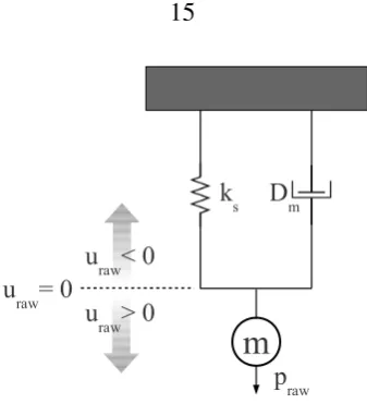
Figure 2.6: Simple harmonic oscillator model of the Agilent Nanoindenter G200 XP head

1 nm.) Load can be applied up to 500 mN with a claimed resolution of 50 nN, far beyond the capabilities needed for these experiments.

By design, the XP head can be modeled as a simple harmonic oscillator as shown in Figure 2.6. In this illustration, ks refers to the spring constant associated with the loading

column and attributable to the leaf springs, Dm is the damping constant of the machine,

largely due to air resistance, and m is the mass of the loading column plus the indenter tip (mostly the column). With the assistance of with a SURF student, Pearl Fung, ks,

Ds, and m were calculated for our system following the procedure in Hay et al. [27].

Briefly, this involves oscillating the indenter head with a constant amplitude sinusoidal load and measuring amplitude and phase shift, φ, associated with the resulting sinusoidal displacement, all while holding the indenter head at a fixed uraw. The magnitude of the

load and displacement oscillations are referred to as the harmonic load, ph, and harmonic

displacement, uh, respectively. We gathered uh and theφ for a series of frequencies, f,

from 1 to 40 Hz and at a series ofuraw from−30µm to +90µm. From this the dynamic

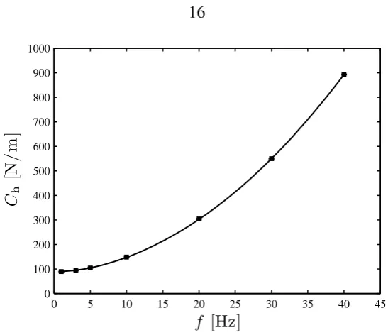
stiffness, Ch = ph/uh is calculated. Finally, ks, Ds, and mare used as fit parameters for

theChversusf data in the simple harmonic oscillator relation [27].

C_h2 = (ks−mω2)2+ (Dmω)2. (2.1)

(29)

0 5 10 15 20 25 30 35 40 45 0

100 200 300 400 500 600 700 800 900 1000

f [Hz]

Ch

[N

/m

[image:29.595.149.423.74.310.2]

]

Figure 2.7: Characterization of the XP head using the simple harmonic oscillator model described by Eq. (2.1) for uraw = 0. Error bars (from four measurements) lie within the

markers. The fit is denoted by the solid line.

at uraw = 0 µm, which illustrates the validity of the simple harmonic oscillator

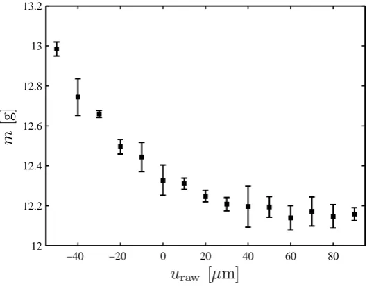
assump-tion. In order to fully understand the system, this test was repeated for a series of raw displacements. A summary of the variation in fit parameters obtained as a function of po-sition, uraw, are given in Figs. 2.8, 2.9, and 2.10. Our results reveal that the system is

most consistently behaved in the range of 0–60µm raw displacement. Thus, experiments are performed within this region in order to obtain the cleanest testing results. Significant changes in the spring constant within this region point to the need to fully account for the machine response, particularly when testing requires a large amount of travel by the inden-ter head and/or when the stiffness of the sample being characinden-terized is on the same order of magnitude as the machine stiffness,ks. These changes arise from the inherent non-linearity

of a real spring. It is for this reason the test methods described in Sections 2.4 and 2.5 perform characterizations in air along with testing the sample.

(30)

can be determined through a plot of the phase angle,φ, the degree by which the oscillatory displacement response lags the load excitation, versus frequency,f. The cutoff frequency is defined at the point where a discontinuity in the phase angle occurs. A plot ofφ(f)(Fig. 2.11) reveals that the cutoff frequency for our system is approximately 50 Hz. Thus, in performing any viscoelastic characterization of our materials, as through the methodology described in Section 2.5, we only utilize frequencies that adhere to the assumption of a simple harmonic oscillator, i.e., those below 50 Hz.

2.4 Microcompression Testing Methods

One of the major reasons for performing uniaxial compression tests is that the load-displacement data gathered during testing can be readily converted into nominal stress and strain in the axial direction. However, before this simple calculation can be performed, the praw and

uraw must be separated into sample and machine contributions. In this section, the

micro-compression experimental procedure is described for performing testing in the XP module of an Agilent Nanoindenter G200 and how the corrected load versus displacement response for the sample only is extracted from the raw data. These procedures are unusually

impor-−40 −20 0 20 40 60 80

12 12.2 12.4 12.6 12.8 13 13.2

uraw [µm]

m

[image:30.595.190.455.487.693.2]

[g]

Figure 2.8: Indenter head mass,m, as a function of raw displacement,uraw obtained from

(31)

−40 −20 0 20 40 60 80 85

86 87 88 89 90 91 92 93 94

uraw [µm] ks

[N/m

]

Figure 2.9: Machine stiffness, ks, as a function of raw displacement, uraw obtained from

the fit of a simple harmonic oscillator model. Error bars were generated from the fit of four separate frequency sweeps at eachuraw.

−40 −20 0 20 40 60 80

2.2 2.21 2.22 2.23 2.24 2.25 2.26 2.27

uraw [µm] Dm

[N/m

s]

Figure 2.10: Machine damping,Dm, as a function of raw displacement,urawobtained from

the fit of a simple harmonic oscillator model. Error bars were generated from the fit of 4 separate frequency sweeps at eachuraw.

(32)

2.4.1 Setting the Sample Up for Testing

Once an array of VACNT pillars has been grown using the methods described in Section 2.2.1.1 or milled using the FIB as described in Section 2.2.1.2, the pillar plus substrate is mounted on a stiff ‘sample puck’ using carbon paint (PELCO Colloidal Graphite, Ted Pella, Inc.) and loaded into the G200 sample tray. Typical microscope to indenter calibration, microscope focal length/sample height, and surface find techniques as described in the G200 user’s manual and applied in the default testing methods are not applicable here due the stickiness and compliance of VACNTs and the geometry of the diamond flat punch indenter tip.

The procedure for bringing the sample to the appropriate height for testing differs from the manual as follows. To get the sample at a height suitable for mechanical testing (i.e., such that testing occurs within the well-behaved range of raw displacement values deter-mined in Section 2.3), a soft polymer sample is first mounted on either a separate puck or the same puck as the VACNT sample. Both PDMS and nail polish were used for this other sample which will subsequently be refered to as the calibration sample. The calibration sample must be soft so that during a microscope to indenter calibration, the large flat punch makes a discernible mark to calibrate against. In the case where the calibration sample is

Cut-off frequency: 50 Hz

(33)

mounted on the same puck as the VACNT sample, the surface of both sample and cali-bration sample must be as close as possible to the same height. In the case that they are mounted separately, the microscope is brought into focus over the fused silica reference sample as described in the G200 user’s manual [29] before moving the calibration sample under the microscope. The sample is brought into focus manually (without using the mi-croscope motor). A Mimi-croscope to indenter calibration reveals the ‘Raw Displacement’ of the surface of the calibration sample. If this is a large number (>100µm) the calibration sample must be raised ‘Microscope to Indenter Calibration’ and the process repeated until the ‘Raw Displacement’ when the surface is found is under 100 µm but greater than20

µm. (The first calibration is likely to occur at a very large raw displacement if the flat punch described in Section 2.2.1.3 is used, as it is much shorter than a standard tip.) Now the calibration sample is near zero ‘Raw Displacement’, the correct height for testing. The microscope focus motor is used to bring the microscope into fine focus on the calibration sample before moving the test sample under the microscope. With the test sample visible under the microscope, the sample puck is raised and lowered manually until it is in focus. Now the sample is at approximately the correct height for performing mechanical tests. The reasons for this procedure are that the calibration sample and the test sample must be at the same height in order for the calibration to be sufficiently accurate and both must be near zero ‘Raw Displacement.’

(34)

small oscillation is applied to the indenter column (ph =10µN) and the harmonic contact

stiffness is monitored by the software. The harmonic contact stiffness measures the elastic part of the dynamic stiffness, Ch, and is corrected within the software for the machine

contribution using a set of tables determined during calibration and setup. Therefore, it hovers near 0±15N/m typically and depending on the amplitude of the oscillation can easily detect changes on the order of 50 N/m, which is the threshold we used for surface determination in these experiments. Because of the relatively high speed of the first test, it must be discarded. However, now the ‘Raw Displacement’ of the VACNT sample is known and is entered as the surface approach starting point along with a slow surface approach speed for all subsequent tests. Note that if the ‘Raw Displacement’ is > 100 µm both the test and calibration samples are raised and the ‘Microscope to Indenter Calibration’ process is repeated to avoid misalignment between the tip and pillar. Further details of the test method are given in Appendix A.

2.4.2 Decoupling Material and Instrumental Response

As the raw load versus raw displacement data collected during nanoindentation experi-ments combines both the material and instrumental responses, careful measures have to be taken in order to accurately decouple the sample-only response and the machine response. This is accomplished through properly modeling the mechanical equivalent of the entire sample-instrument system [30–32]. The equivalent mechanical model of the nanoindenter plus sample for the system of relevance is shown in Fig 2.12. Raw load data (praw),

de-termined by the inductive loading coil, and raw displacement data (uraw), gathered by the

(35)

leaf springs of stiffness,ks, shown in Fig. 2.12), which is slightly position dependent over

large distances (enough to result in a 0.05 mN force difference over some regions of raw displacement, which is around 0.1% of the total load obtained). Post-processing (not in Testworks) interpolates between the values ofps taken at 10 locations within the

displace-ment regime and uses this information to removepsfromprawat every time point. Finally,

there is a small contribution to the force by the machine damping (Dm), which is calculated

during the post-test characterization in air. However, this latter contribution is marginally important for only the highest strain rates, ˙n, tested (displacement rates, u˙) of 0.1 and

0.5 s−1 where the force,Dmu˙, is on the order of 0.05 mN. The resulting equation for the

corrected load on the indenter tip/load frame/sample assembly (solid boxed region of Fig. 2.12),pcorr, is therefore

pcorr =praw−ps+Dmu.˙ (2.2)

It follows that the load on the sample is simply the load on this assembly due to the fact that these three elements are in series. The corrected displacement (ucorr), i.e., the actual

displacement applied to the sample, accounts for the deformation in the load frame (frame stiffness,kf) and the diamond indenter head (stiffness,ki). Again, since the sample, frame,

m

k_i

k₁

k₂

k_s

D_c

D_m k_f

sample (as SLS)

p_raw

sample + indenter/frame assembly

Figure 2.12: Viscoelastic model of the nanoindenter plus sample system utilized to obtain the correct load on the sample from the measured load, praw. For most calculations, the

(36)

and indenter head are in series (Fig. 2.12), the corrected displacement can be written as

ucorr =u−

pcorr

kf

−pcorr

ki

, (2.3)

wherekf for our system is5.92×106N/m (calculated during instrument setup and

calibra-tion) andkiis calculated from the known elastic modulus,ED, and Poisson’s ratio,νD, of

diamond. The relationship for determiningkiis [30]:

ki =

2ED

(1−ν2 D)

p

Ai/π

, (2.4)

whereAi is the cross-sectional area of the indenter area in contact with the sample. Both

corrections turn out to be inconsequential (∼0.01nm) for such a compliant material under such large deformation. Additional corrections could be imagined for the compliance of the Si wafer on which the pillar sample is mounted or the carbon paint attaching the wafer to the puck, but, as is evident from the corrections for frame and indenter tip compliance, these would be minor, on the scale of random noise in the displacement signal.

As discussed in detail in the previous section, surface contact is marked by attaining a 50 N/m threshold in the harmonic contact stiffness, as a threshold any lower than that has been found to result in a significant number of false positives for surface contact due to the mechanical and electrical noise. It is important to recognize that crossing this threshold represents the initial contact, likely caused by several stray tubes or a slight misalignment between the flat pillar surface and flat punch rather than by full cross-sectional contact; full contact usually occurs within 0.5µm of raw displacement from that point. Upon establish-ing contact, the harmonic measurement option can be turned off before proceedestablish-ing with the compression. For the results in Section 4.2 this was done due to the fact that the indenter head cannot be oscillated fast enough to provide meaningful data at the faster displacement rate used. We identify the first attainment of full contact in post-processing by locating the first occurrence of a tangent slope in thepcorr versusucorr data of 10 N/m in order to have

a consistent surface threshold for all tests. This value corresponds to a marked increase in

pcorr relative to the maximum load attained in the quasi-static tests. Utilizing the correct

(37)

that point for a zero stress zero strain initial value. It should be noted that,pcorris already

approximately zero at this point, being less than 0.04 mN while the maximum pcorr

ap-proaches 40 times this value providing verification that our surface find and data correction procedures are accurate.

In the experiments described in this thesis, the nanoindenter compresses the samples at a constant, prescribed raw displacement rate (u˙raw), and therefore a constant nominal

sam-ple strain rate, throughout the entire experiment (loading and unloading). Examsam-ples of the instrument’s response to the prescribed displacement rate schedules are shown in Fig 2.13.

load ing 67 nm/s

32.85 µm/s 6.67 µm/s

unloading

loss of surface contact

(38)

Recall from Section 2.3 that the G200 is inherently load controlled, which means that con-stant displacement rate tests invoke the use of proportional control with limits on maximum and minimum loading rates. During a constant displacement rate uniaxial compression, the loading schedule, ucorr(t), where t is time, is ideally a straight line with slope equal to

the prescribed rate. The displacement schedules for the two slowest rates we utilized have nearly perfect control (straight lines), while the two fastest rates show a progressive de-crease in control, illustrating the limitations of the inherently load controlled nanoindenter. The maximum percent errors associated with the prescribed displacement rates used were 2×10−3_{% for the slowest rate and 0.25% (up to 0.4% for beginning of unload) for the}

fastest rate. These are very minor errors and the tests can be assumed to be constant strain rate.

2.4.2.1 Compression Method Details

(39)

2.5 Microscale Dynamic Testing Methods

Dynamic testing methods, in which samples are subjected to oscillatory loads or displace-ments, are typically used in the characterization of viscoelastic materials. These materi-als exhibit both viscous/ energy-dissipating and elastic/energy-storing characteristics when subjected to load. Viscoelastic behavior is generally quantified in terms of the storage,

E0, and loss, E00, moduli which are the real and complex parts, respectively, of the com-plex modulus (or by the ratio, tanφ, of these two moduli). The modulus, however, is not the most fundamental measurement of the viscoelastic response. It is calculated from the harmonic stiffness, Ch, which is the ratio of the harmonic load and displacement

am-plitudes, ph/uh. Conversion between harmonic stiffness and complex modulus is

accom-plished through the well known Sneddon relation, [33]

E =Ch √

π

2β

1−ν2

√

A , (2.5)

and requires knowledge of a material’s Poisson’s ratio,ν; unmeasured for VACNTs. It is for this reason I calculate only storage and loss stiffnesses rather than storage and loss moduli in characterizing the viscoelastic properties of VACNTs. In Eq. (2.5),β is a constant that depends on the indenter geometry (1 for a flat punch) andA is the contact area (∼2,500

µm2).

In a typical dynamic testing experiment, the material is loaded to a desired strain and the mechanical probe is oscillated across a range of frequencies. By measuring the resultant load amplitude, displacement amplitude, and the phase lag during the test (following the methods outlined in Herbert et al. [28] and Wright et al. [32]), the values of loss stiffness (kloss) , storage stiffness (kstorage), and tanφ are determined. This method is identical to

the dynamic mechanical analysis (DMA) of polymers, but occurs at a much smaller scale in terms of both oscillation amplitude and sample size. Specifically, I gather the storage and loss stiffnesses by oscillating the indenter head at ∼8 nm amplitude while sweeping the frequency from 1 to 45 Hz while holding the nominal strain constant at 10 values: from 0.01 to 0.8.

(40)

et al. [32] prescribe removal of the machine contribution by performing a second set of measurements in air (at the same raw displacement). Therefore, the storage and loss moduli for the sample/frame assembly are written

kstorage =

ph uh

cosφ−

ph uh air

cosφair, (2.6)

kloss =

ph uh

sinφ−

ph uh air

sinφair. (2.7)

Here the subscript ‘air’ refers to the measurements taken while the head oscillated in air (i.e., not in contact with the sample). While this method treats the entire sample/frame assembly as a black box, a positive aspect of this treatment is that these stiffnesses remain independent of the indenter mass. This is important as values calculated for the indenter head mass utilize several assumptions and can be somewhat variable as shown in Section 2.3. It is reasonable to assume that stiffnesses calculated via Eqs. (2.6) and (2.7) correspond to those of the sample since both the frame and the indenter head stiffnesses are several orders of magnitude higher than those of the sample and thus can be assumed to be infinite [28]. It should be noted that a channel in Testworks referred to as the ‘Harmonic Contact Stiffness’ is essentially equivalent to kstorage. The only difference in this instance is that

I characterize the behavior of the indenter head in air each time I perform a test and the ‘Harmonic Contact Stiffness’ channel uses tabulated values for the stiffness in air used in Eqs. (2.6) and (2.7). For highly compliant materials, characterization after each test yields more accurate results. The Testworks method utilized in this thesis for dynamic mechanical analysis is detailed in Appendix B.

2.6 In Situ

Testing Setup

(41)

in the data, thus it is our ‘mentor.’

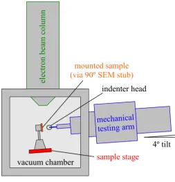
Samples to be tested are mounted on a 90 degree SEM stub and loaded into the SEM chamber at a tilt of 4 degrees from vertical. The mechanical testing arm is mounted on a side port of the SEM (FEI Quanta 200) at an angle of 4 degrees from the horizon. The geometry is illustrated in the schematic in Figure 2.14 with photos of the actual system given in Figure 2.15. The mechanical arm is a derivative of the technology in the DCM head of the Agilent Nanoindenter G200 and is therefore subject to the same limitations. The first limitation is in the raw displacement which ranges from−15to +15µm. Also, maximum attainable load is 10 mN with a resolution of 50 nN. The maximum load is sufficient for our tests, but because of the limited raw displacement, in situ testing of 60

µm tall VACNT pillars is limited to nominal strains of only 50%.

el

ec

tr

on

b

ea

m

c

ol

um

n

mechanical testing arm

sample stage

4º tilt

vacuum chamber

mounted sample (via 90º SEM stub)

[image:41.595.160.414.342.606.2]

indenter head

Figure 2.14: Schematic of thein situtesting instrument, SEMentor.

(42)

Figure 2.15: Photo of the in situ testing instrument, SEMentor [34]. The image on the left is the complete system with the mechanical testing arm shielded from environmental influences. The image on the upper right is a few inside the SEM chamber. The image on the lower right is the nanomechanical testing arm before shielding has been installed.

‘Support Spring Stiffness’ channel, which is a table of leaf spring stiffness values as a function of raw displacement, ks,table(uraw), obtained during a calibration run. This data

is quite noisy, so the channel must be collected during thein situcompression, smoothed, then removed from the applied load yielding an approximate load on sample,

pcorr =praw(uraw)−praw,surf−(uraw−uraw,surf)ks,table(uraw), (2.8)

where the subscript ‘surf’ refers to value at the point of surface contact. This correction is necessary because of the large position dependence of ks,table, which would otherwise

(43)

Chapter 3 Characterization of VACNT Morphology

3.1 Introduction

(44)

high magnification SEM images taken of the pillar surface at evenly spaced heights along the pillar axis in Fig. 3.1. Quantification of this gradient has only been reported for high energy synchrotron measurements of bulk CNT films as they grow [35], a method that is both expensive and inapplicable to our sample geometry. For this reason, in Section 3.2 I discuss the image analysis techniques developed to analyze this relative density gradient directly from the SEM micrographs. These techniques are developed in collaboration with Peter Capak of the Spitzer Science Center at Caltech.

500 nm 10 µm

Figure 3.1: Cylindrical pillar with32,000×magnification insets, revealing the highly inho-mogeneous CNT microstructure from bottom to top. The lower leftmost image corresponds to the bottom of the pillar and illustrates the sparser (less dense) and less vertically aligned CNTs when compared to the top of the pillar (upper rightmost image). Note that the surface tubes appear brightest because they return more signal to the electron detector, but these tubes are not indicative of the internal pillar microstructure and should be looked beyond in order to observe the density and alignment variation discussed.

(45)

were characterized by transmission electron microscope (TEM) (see Fig. 3.2). Diameters are found to vary between 15 and 30 nm with 22 nm being the average value. The tubes themselves are multiwalled, typically comprised of 4–5 walls per tube. Average density is clearly an important feature in comparing the mechanical response of any foam-like mate-rial. For example, the elastic modulus of a foam scales with the relative density squared for foamed metals and polymers [23], where relative density is the foam density divided by the density of a single, monolithic strut. Similar relationships exist for energy dissipation and plateau stress. Unfortunately, determining either the average tube number density or mass density has proven challenging due to the small size of individual pillars (lack of material for bulk measurement) and the large amount of open space (small surface area per gram of sample). Attempts to determine the density of the samples tested are discussed in Section 3.3.

20 nm 10 nm

Figure 3.2: TEM images illustrating the typical multiwall CNTs making up the VACNT bundles tested. There are typically 4–5 walls per tube. Images taken by A. T. Jennings.

3.2 Density Gradient

(46)

catalyst is lost during the growth process (carried away by the tubes themselves or diffused into the substrate) less CNTs are being produced. The CNTs that have already been grown, however, are carried/pushed away from the substrate as new CNTs continue to form and grow. Knowing the gradient in number density that arises from this growth process is

cen-1 2 3 4 5

1 2

3 4

5

200 nm

Figure 3.3: A series of SEM images at distances of 1) 5 µm 2) 15 µm 2) 25 µm 2) 35

(47)

tral to understanding the overall structural material response of the VACNTs under load. It is also necessary in order to separate that overall response from the local material response.

SEM images are relatively easy data to acquire for any VACNT system regardless of density, tube diameter, or size of the film. For this reason, I have made efforts to analyze several series of images (a single series corresponds to a set of images along the height of the CNT pillar) in order to quantify therelativedensity differences between them. Note that an absolute density cannot be obtained from an SEM image in this case as the interaction volume is unknown. In fact, calculation of the interaction volume is extremely complicated due to the porous nature of VACNTs. In attempting to differentiate the number of tubes between two micrographs, the issue of image normalization becomes apparent. Thresh-olding, in which all pixels above a given saturation value are made white and all those below are made black, appears at first to be the most straightforward way to determine the number of tubes in an image [37]. However, the images do not have the same contrast or brightness values as these values were manually tuned along the height of the pillar in order to retain information (i.e., the same brightness and contrast settings at the bottom of the pillar would result in a completely black image at the top). Therefore, the threshold must be set for each individual image, a non-trivial task in which it is difficult to deconvo-lute the brightness and contrast of an image’s histogram from the tube density contribution to the histogram. Briefly, brightness is defined as overall saturation of an image or where it falls on the grayscale from 0 to 255. Contrast is roughly defined as the breadth of the image histogram; approximately the maximum pixel value less the minimum pixel value. A typical SEM micrograph with its corresponding histogram are given in Figs. 3.4(a) and (c). Based on the wide variation in brightness and contrast observed between experimental images, it can be concluded that the images must be either normalized with respect to both or a method must be found that is insensitive to these image properties while still being sensitive to the structure found within an image.

(48)

va-lidity of a method throughout its development, A series of simulated tube images having characteristics analagous to the experimental images is generated. Once these simulation

c)

a) b)

d)

e)

(49)

images produce meaningful trends for a given method, limitations of the image analysis technique can be explored through controlled deviations from the experimental character-istics. Subsequently, a figure of merit corresponding to the relative increase in tube number can be developed. For this reason, key features of the experimental SEM images must be measured.

3.2.1 Experimental Image Characterization

Careful measurement of the tube diameter, image noise, and relative tube and image satu-ration values is performed. Tube diameters are measured by hand/eye using the software ImageJ. The resulting distribution of diameters is given in Fig. 3.5(a). The data is more reasonably fit with a log-normal distribution than a Gaussian. The average tube diameter is

a)

b)

(50)

22.3 nm with a mode of 21.1 nm and log-normal standard deviation of 0.31. Analagously, tube saturation data is gathered by taking the average value from a region of each of the tube encountered while progressing horizontally across an image. This data is presented in Fig. 3.5(b) and fit with a Gaussian distribution having a mean of 162 and standard deviation of 22 (out of a scale from 0 to 255). As each of these data analyses are tedious and many data points were collected, they were performed for only one experimental image. It is reason-able to assume that tube diameter is not changing significantly (and indeed does not appear to do so) between images. The standard deviation of tube intensity or saturation value will certainly change with image contrast, but, as stated earlier, that must be accounted for in the method deveoped. The most important attribute to bear in mind for tube intensity is that it has a Gaussian distribution and thus this will be a key feature of the simulated images.

Image noise is measured by calculating the standard deviation of pixel values within a relatively homogeneous subregion of the image. It is found to increase slightly with increasing local intensity which is expected. This is because the noise can likely be char-acterized as shot noise, i.e., due to the finite nature of the electrons interacting with the detector, which is proportional to the square root of the mean saturation or intensity of a pixel. The average noise (taken as the standard deviation of the pixel saturation values) for the SEM images is 0.02 ±0.005. This value is not a function of the height at which the image is taken. Implementation of the characteristic tube diameter, brightness distribution, and noise in a series of simulated images is given in Appendix D. A typical simulated image and its corresponding histogram are shown in Figs. 3.4(b) and (d).

3.2.2 Pattern Extraction with the Power Spectrum

(51)

contains no absolute position information, only relative position information. Thus, it can be used to measure the presence of structure at a certain lengthscale in the image. Typical power spectra obtained for experimental and simulated images are shown in Fig. 3.4(e). By convention, small wavelength or spatial scale is on the right and corresponds to pixel to pixel variation. The power at this lengthscale generally reflects the contrast of the image. However, I have found that it is also convolved with the tube number density and there-fore cannot be used to normalize the power spectra between multiple images. Note that the power signal rises sharply around a wavelength of 10 pixels, which corresponds to the approximate diameter of an average CNT.

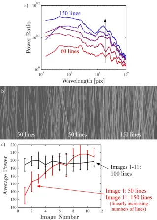
Using the power spectra, one can explore changes in power response to changes in the image’s characteristics. Two series of simulated images (having characteristics similar to the experimental images as determined by the data presented in Section 3.2.1) are generated such that the contrast (and brightness, though it has no effect on the power spectrum) of each image was identical:

S1: 10 sets of 11 images - linear variation in line number from 50 to 150

S2: 10 sets of 11 images - no variation in line number, 100 lines in each

(52)

required to measure changes in the amount of fibrous structure within these experimental images, particularly within the tube number range of interest.

Additionally, when the same methods are used on a series of images in which the bright-ness and contrast of the simulated images is varied randomly, all correlation is lost. This

Image 1: 50 lines Image 11: 150 lines

(linearly increasing numbers of lines) Images 1-11: 100 lines

50 lines 50 lines 150 lines

60 lines

150 lines a)

b)

[image:52.595.166.486.197.644.2]

c)

(53)

is because the contrast in the images has not been normalized. As a result, several contrast regularizing techniques were attempted: normalizing by the shortest wavelength, normaliz-ing by the gain, and normaliznormaliz-ing by the contrast as determined by the image histogram. At this time, a correct or experimentally feasible normalizing procedure has not been found.

a) b)

c)

d)

[image:53.595.73.506.254.698.2]

200 nm 100 pixels

(54)

3.2.3 Edge Detection

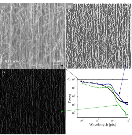
Another typical image analysis method generically known as ‘segmentation’ involves lo-cating edges or objects of interest within an image. One issue with a typical edge find technique can be finding edges at lengthscales that are not of interest or missing edges due to changes in contrast either locally or between images when a threshold is set inappro-priately. Since the region of the power spectrum corresponding to signal from the tubes is known, we can mitigate these issues by first filtering the image in the frequency domain with respect to this lengthscale. This results in an image in which the structure of interest is brought to the forefront. An example of a Gaussian bandpass filtered image in which a his-togram normalization procedure has been performed to highlight the remaining structure is shown in Fig. 3.7(b). For reference the high contrast, but otherwise unaltered filtered result is shown in Fig. 3.7(c). Corresponding radially averaged power spectra in Fig. 3.7(d) verify the emphasis on the tube-scale structure present in the filtered image. Future efforts will be focused on the appropriate selection of filter and subsequent edge detection method in order to develop a method that is robust under changes in both contrast and brightness between images while giving resolution in line number density.

3.3 Material Density

It is generally taken for granted that a material’s density and volume fraction, in the case of porous materials, can be easily obtained. For nanoscale and nanostructured materials how-ever, this is not always true. Our VACNT pillars are both. In bulk specimens of VACNTs the density,ρVACNT, and volume fraction of tubes,φCNT, can be readily measured using a

mass balance, the volume of the weighed sample,Vtotal, and the known density of graphite,

ρgraphite = 2.2g/cm3, via the relations,

ρVACNT =

m Vtotal

φCNT =

m/ρgraphite

Vtotal

=ρVACNT/ρgraphite. (3.1)

(55)

How-ever, the size of our VACNT pillars does not allow for such simple techniques. A 1 cm×1 cm continuous film of VACNT having a height similar to that of the VACNT pillars tested here (60µm) weighs only 0.66 mg. This is not feasibly measurable on a typical lab scale and requires measurement using a high sensitivity mass balance, such as that used in ther-mogravimetric analysis (claimed resolution of ∼1 µg). To complicate things, the weight of the Si substrate on which the samples are grown is several orders of magnitude larger, making the sample’s removal from the substrate necessary for measurement. Practical lim-itations make this undesirable: The sample is destroyed and brittle flaking occurs to such an extent that the VACNTs cannot be completely harvested. For this reason, we attempted to utilize a technique commonly applied to highly porous materials, nitrogen adsorption, following the Brunauer-Emmett-Teller (BET) theory for analysis of the results.

Briefly, BET theory is a multilayer extension of Langmuir theory, which is itself a theory for monolayer molecular adsorption of gas onto a surface. Measurements of the amount of gas adsorbed onto the sample surface at a given supersaturation combined with known quantities of the size of the gas molecule result in the ability to perform a calculation of the surface area of a sample. Systems capable of BET measurements typically require samples having a surface area of 0.1 m2to∼300 m2, e.g., catalyst materials like zeolites or adsorbants like activated carbon. Once a surface area measurement is obtained, an estimate of the porosity, given average values for the average inner,di ≈7nm, and outer,do ≈20

nm, radii of the CNTs (combined with the assumption that N2 adsorption occurs on both

the inner and outer surfaces), can be calculated via the relation

φ= d

2

o −d2i

do+di

Asurface

4Vtotal

. (3.2)

This estimate is still sensitive to measurements of the sample volume, but determination of the mass has been eliminated. Unfortunately, for a 1 cm×1 cm×60µm sample with an estimated volume fraction of 0.05 (from bulk), one can only expect surface areas of∼0.1, which are at the low end of the measurement capabilities for the N2 adsorption instrument

(56)

(57)

Chapter 4 Deformation Under Uniaxial

Compressive Loading

4.1 Introduction

(58)

bun-dles compressed in an SEM using an Omniprobe [46]. Many of the qualitative descriptions we observe here were reported, however, the mechanical probe had no load or displacement sensors such as characterize ourin situtesting setup. Some of these materials display a high recoverability after significant strain, even after cyclic loading [24], while others have been observed to deform permanently [15, 44, 46]. This thesis explores the largely irrecoverable deformation we observed upon uniaxial compression of the VACNT bundles. The results presented within this chapter were first published in Hutchens et al. [44].

Uniaxial microcompression experiments were selected as the mechanism for studying the mechanical properties of VACNTs for reasons of simplified analysis as well as for the fact that a free surface allows for observation of the rich morphological response charac-terized by sequential, periodic folds or buckles as we will refer to them hereafter. While nanoindentation tests on VACNT films [14, 42] and on photolithographically defined fea-tures [15, 16] have provided tangent and elastic moduli, they cannot explore this wrinkle-like morphology due to its highly localized nature and the limited overall strain that can be analyzed in this testing geometry. In this chapter, we present our observations of the morphological evolution and corresponding mechanical response seen in cylindrical, 50

µm diameter CNT foam bundles subjected to uniaxial compression at different strain rates. We chose to test 50 µm diameter pillars with an aspect ratio of 2.4–2.8 (height/radius) because they are large enough to produce multiple surface undulations, as observed previ-ously [15, 24], while being small enough to capture the local deformation events that occur during compression in our custom-built in situ mechanical deformation system, SEMen-tor [34] (see Section 2.6). Fortuitously, testing such small samples also enables resolution of the local buckling events within the overall stress-strain response, as will be shown in Section 4.2.

(59)

(60)

Table 4.1: Table of Published Values for the Elastic Modulus of VACNTs

E (MPa)

Measurement

Method Density Reference

50 Uniaxial compression 0.3 g/cm3 a Cao, et al., 2005 [24].

∼50 DMA NG Mesarovic, et al., 2007

[42].

<2 Uniaxial compression NG Suhr, et al., 2007 [20]. 0.25 Uniaxial compression

- loading

1010_cm−2 b _{Tong, et al., 2008 [45].}

15

Nanoindentation (Berkovich) -unloading

NG Zbib, et al., 2008 [15].

18,000 Nanoindentation (flat punch) - loading

0.95 g/cm3 Pathak, et al., 2009

[14].

∼1 DMA 0.009 g/cm3 Xu, et al., 2010 [19].

58

NG Zhang, et al., 2010 [47].

50±25b

NG* Qiu, et al., 2011 [43].

a _{Reported as an 87% porosity estimate, converted to approximate density using the}

density of graphite.

b _{Tube areal number density (20–30 nm diameter CNTs).}

b _{Reported as a reduced modulus. Indentation was performed with a diamond tip, so}

difference from actual sample modulus is small.

Deformation Behavior and Mechanical Analysis of Vertically Aligned Carbon Nanotube (VACNT) Bundles

ANALYSIS OF VERTICALLY ALIGNED CARBON

NANOTUBE (VACNT) BUNDLES

Shelby B. Hutchens

Acknowledgements

Abstract

Contents

List of Figures

List of Notation

Chapter 1

Introduction

1.1

Definition and General Characteristics of Vertically

Aligned Carbon Nanotubes

Anisotropic

Isotropic

Discrete

1.2

Applications

1.3

Objectives and Scope

Chapter 2

Experimental Procedure

2.1

Introduction

2.2

Sample and Nanoindenter Tip Fabrication for

Uniax-ial Testing

2.2.1

VACNT sample preparation

2.3

Characterization of Micromechanical Testing System

m

2.4

Microcompression Testing Methods

2.4.1

Setting the Sample Up for Testing

2.4.2

Decoupling Material and Instrumental Response

m

2.5

Microscale Dynamic Testing Methods

2.6

In Situ

Testing Setup

Chapter 3

Characterization of VACNT Morphology

3.1

Introduction

3.2

Density Gradient

3.2.1

Experimental Image Characterization

3.2.2

Pattern Extraction with the Power Spectrum

3.2.3

Edge Detection

3.3

Material Density

Chapter 4

Deformation Under Uniaxial

Compressive Loading

4.1

Introduction