An evaluation of analytical stream to groundwater exchange models: a comparison of gross exchanges based on different spatial flow distribution assumptions

www.hydrol-earth-syst-sci.net/18/2715/2014/ doi:10.5194/hess-18-2715-2014

© Author(s) 2014. CC Attribution 3.0 License.

An evaluation of analytical stream to groundwater exchange

models: a comparison of gross exchanges based on different

spatial flow distribution assumptions

M. Exner-Kittridge1, J. L. Salinas2, and M. Zessner3

1_{Centre for Water Resource Systems, Vienna University of Technology, Vienna, Austria}

2_{Institute of Hydraulic Engineering and Water Resources Management, Vienna University of Technology, Vienna, Austria} 3_{Institute of Water Quality, Resources and Waste Management, Vienna University of Technology, Vienna, Austria} Correspondence to: M. Exner-Kittridge ([email protected])

Received: 28 June 2013 – Published in Hydrol. Earth Syst. Sci. Discuss.: 15 August 2013 Revised: 27 May 2014 – Accepted: 16 June 2014 – Published: 29 July 2014

Abstract. In this paper, a new method for estimating gross

gains and losses between streams and groundwater is devel-oped and evaluated against two existing approaches. These three stream to groundwater exchange (SGE) estimation methods are distinct in their assumptions on the spatial dis-tribution of the inflowing and outflowing fluxes along the stream. The two existing methods assume that the fluxes are independent and in a specific sequence, while the third and newly derived method assumes that both fluxes occur simul-taneously and uniformly throughout the stream. The analytic expressions in connection to the underlying assumptions are investigated through numerical stream simulations to evalu-ate the individual and mutual dynamics of the SGE estima-tion methods and to understand the causes for the differences in performance. The results show that the three methods pro-duce significantly different results and that the mean absolute normalized error can have up to an order of magnitude dif-ference between the methods. These difdif-ferences between the SGE methods are entirely due to the assumptions of the SGE spatial dynamics of the methods, and the performance for a particular approach strongly decreases if its assumptions are not fulfilled. The assessment of the three methods through numerical simulations, representing a variety of SGE dynam-ics, shows that the method introduced, considering simulta-neous stream gains and losses, presents overall the highest performance according to the simulations. As the existing methods provide the minimum and maximum realistic val-ues of SGE within a stream reach, all three methods could

be used in conjunction for a full range of estimates. These SGE methods can also be used in conjunction with other end-member mixing models to acquire even more hydrologic in-formation as both require the same type of input data.

1 Introduction

Groundwater and surface water interactions are an important process in hydrologic systems (Winter, 1998). These interac-tions within and around streams and rivers impact decisions on municipal water supply extractions, water pollution, river-ine habitat, and many others. To make better decisions on these impacts, the stream to groundwater exchange (SGE) needs to be accurately quantified as stream losses and gains can account for a substantial proportion of the total flow and chemical load of a stream.

2716 M. Exner-Kittridge et al.: Stream to groundwater exchange models

gains and losses into and out of the stream can be very dy-namic even over short distances (Harvey and Bencala, 1993; Anderson et al., 2005; Payn et al., 2009). Consequently, what might have originally been estimated as a small gain to the stream from simply subtracting the upstream and down-stream discharges might end up becoming a small loss out of the stream and a large gain into the stream. Without a proper method to estimate SGE, any attempt at estimating a water or nutrient mass balance would be difficult and laced with errors.

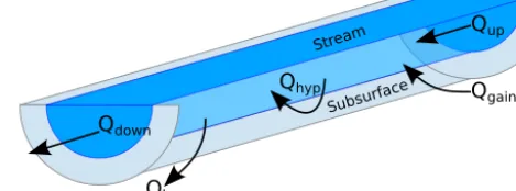
Harvey and Wagner (2000) and many other researchers use a more realistic conceptual model of flow pathways within a stream (Fig. 1). These major flow pathways include initial (or upstream) discharge (Qup), final (or downstream) discharge (Qdown), stream gains from groundwater (Qgain), stream losses to groundwater (Qloss), and hyporheic flow (Qhyp). In this conceptual model,Qgainis considered to be pure ground-water entering the stream, and Qloss is stream water per-manently leaving the stream. Hyporheic flow occurs when stream water temporarily leaves the stream into the surround-ing groundwater (or more specifically the hyporheic zone), but returns again to the stream at some downstream location. During this temporary departure from the stream, additional biochemical reactions may occur that would not necessarily have occurred while in the stream itself. The mass is still re-tained in the stream and not lost (permanently) to the ground-water. Although the hyporheic flow pathways do occur and can be very important for stream ecosystems (e.g., the move-ment of oxygen into the hyporheic zone, nitrogen cycling, etc.), hyporheic flow will not be directly addressed in this study as the authors are most interested on fluxes that are per-manently adding or removing mass over a significant length of stream. As hyporheic flows only temporarily leave the stream, the mass of the water is still retained over sufficient distances.

There are a number of methods to estimate gross stream gains and losses (Kalbus et al., 2006). The general cate-gories are seepage meters, (heat or chemical) tracer tests, and hydraulic gradients derived from groundwater piezometers. Each has advantages and disadvantages. Seepage meters and groundwater piezometers are point measurements that can be accurate at a specific point, but in a heterogeneous sys-tem they may not represent the stream as a whole. However, chemical tracer tests are an aggregation of all fluxes along a stream reach, but do not represent any particular point along the stream. For this study, the focus is on the total aggregated flows over the stream reaches, so chemical tracer tests were found to be the most appropriate and inexpensive. Kalbus et al. (2006) and Scanlon et al. (2002) have a more thorough qualitative review of the different SGE methods.

Using chemical tracer tests for the source of data, the es-timation of gross stream gains and losses is most frequently performed through numerical models like those similar to the OTIS (One-Dimensional Transport with Inflow and Storage) model developed by the USGS (United States Geological

Qgain

Qloss

Qup

Q_down

Qhyp

Stream

Subsurface

Figure 1. A conceptual overview of the major inflows and outflows

within a stream reach.Qupis the upstream discharge in volume per

time,Qdownis the downstream discharge,Qgainis the groundwater

entering the stream,Qlossis the stream water leaving the stream to

the groundwater, andQhypis the hyporheic flow water that is

tem-porarily leaving the stream into the hyporheic zone. (Reproduced after Harvey and Wagner, 2000.)

Survey) (Runkel, 1998). While able to estimate fluxes in steady-state conditions, these types of models are primarily designed for non-steady-state conditions and provide many output parameters in addition to the inflow and outflow fluxes and, as a consequence, require more input data than in steady-state conditions for estimating only SGE (e.g., stream cross-sectional area, flow advection, flow dispersion, etc.). Additionally, the OTIS type models would require the esti-mation of parameters, through a trial-and-error or an auto-mated nonlinear least-squares (NLS) procedure, that are not directly measured. Under steady-state conditions, the data and parameter requirements for estimating only SGE are sub-stantially lower requiring only discharge and tracer concen-tration measurements upstream and downstream. If a steady state is appropriate, then analytical methods are sufficient.

There are two existing analytical methods to estimate SGE under steady-state conditions ignoring hyporheic flow paths. These methods use simple mass balance equations to esti-mate both gains and losses within a stream reach and assume that the fluxes are independent and in a specific sequence. In this paper, a new analytical method has been developed using different assumptions on the spatial distribution of the inflowing and outflowing fluxes along the stream. The new spatial distribution assumptions are simultaneous and uni-form inflows and outflows over the entire stream reach.

2 Methods

2.1 Theoretical basis of the SGE tracer methods

All tracer based methods designed to estimate SGE start with the conservation of mass equations under steady-state condi-tions for both the tracer and the water flux and assume com-plete mixing of the individual flows:

QupCup+QgainCgain=QdownCdown+QlossCloss, (1)

Qup+Qgain=Qdown+Qloss, (2)

where Qdown is the downstream discharge (in volume per unit time), Cdownis the downstream concentration (in mass per unit volume), Qup is the upstream discharge, Cup is the upstream concentration,Qgainis the discharge from the groundwater to the stream, Cgain is the concentration of Qgain,Qlossis the discharge from the stream to the ground-water, andClossis the concentration ofQloss.

If we assume that Cgain will be estimated later from the tracer test, then there are three unknown variables (i.e.,Qgain, Qloss, andCloss) and two equations. As we want to solve for QgainandQloss, we must make some assumption aboutCloss to make the derivation solvable. The two existing SGE esti-mation methods mentioned in the introduction make specific assumptions on the distribution of gains and losses through-out the reach (see Fig. 2) to make appropriate assumptions aboutCloss. The first method, we call “Loss–Gain” assumes Closs=Cup, while the second method, we call “Gain–Loss”, assumesCloss=Cdown. In both variants, the methods assume that the mixing ofQgainCgainandQlossClossare mixed sep-arately and in a sequence defined by the above assumptions. The Loss–Gain variant assumes that the mixing sequence begins with Qloss followed by Qgain, while Gain–Loss is vice versa.

Combining Eqs. (1) and (2), the solution for Qloss for Loss–Gain is

Qloss,LG=Qup−Qdown _C

down−Cgain Cup−Cgain

. (3)

Similarly, the equation forQlossfor Gain–Loss is Qloss,GL=Qup

_C

up−Cgain Cdown−Cgain

−Qdown. (4)

To get Qgain for both methods, we need to include Eq. (2) into Eqs. (3) and (4):

Qgain,LG=Qdown _C

down−Cup Cgain−Cup

, (5)

Qgain,GL=Qup _C

down−Cup Cgain−Cdown

. (6)

If we use an artificial tracer (e.g., bromide salt), we can safely assumeCgain≈0 and the resulting equations are as follows: Qloss,LG=Qup−Qdown

Cdown Cup

, (7)

Qgain Qloss

Qup

Qdown

Loss-Gain Gain-Loss

Qgain

Qloss Qup

Qdown

Simultaneous

Qgain Qloss

Qup

Qdown

A B C

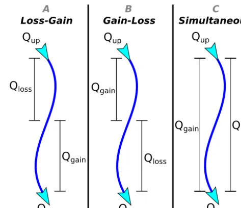
Figure 2. The conceptualizations of the three SGE methods.

(A) The LG (min) method assumesQgainoccurs in the first section

followed byQloss in the last section. (B) The GL (max) method

assumesQlossoccurs in the first section followed byQgainin the

last section. Both the LG (min) and GL (max) methods assume that

QgainandQlossoccur in sequence and independently, although the

lengths of the first and last sections are arbitrary and can be of any length that when summed together equal the total length. (C) The

SIM method assumes thatQgainandQlossare constant and occur

simultaneously throughout the entire length of the stream reach.

Qloss,GL=Qup Cup Cdown

−Qdown, (8)

andQgainbecomes

Qgain,LG=Qdown

1−Cdown

Cup

, (9)

Qgain,GL=Qup _C

up Cdown

−1

. (10)

These methods can be applied conceptually along a stream length as illustrated in the A and B sections of Fig. 2.Qup is the upstream discharge andQdown represents the down-stream discharge. Depending on the equation variant,Qgain is added orQlossis removed fromQupat the beginning of the stream andQlossis removed orQgainis added at the end of the stream resulting in a downstream discharge ofQdown. As these methods make no assumptions about the exact location along the stream forQgainandQloss, they can occur over any length of the stream as long as they occur in sequence and independently.

2718 M. Exner-Kittridge et al.: Stream to groundwater exchange models

changing towards the concentration ofCgainwheneverQgain enters the stream, and finally ending downstream at a value of Qdown (which again is a value towards that ofCgain). As this occurs in every possible stream reach where Qgain>0 andCgain6=Cup6=Cdown,Cup andCdown represent the end-point concentrations along a stream reach. Subsequently, the Loss–Gain (with theCup assumption) and Gain–Loss (with theCdown assumption) methods represent the minimum and maximum possible SGE values given the initial mass balance assumptions from Eqs. (1) and (2). This also means that any other SGE method must result in SGE values between the Loss–Gain and Gain–Loss methods. To provide the reader with an intuitive sense of both the underlying spatial distri-bution assumptions and the end point that these two methods represent, the Loss–Gain method will be called “LG (min)” and the Gain–Loss method will be called “GL (max)”.

From studies that tested multiple stream reaches for SGE, almost every stream reach had both gains and losses regard-less of the method and of the reach length (Anderson et al., 2005; Ruehl et al., 2006; Payn et al., 2009; Covino et al., 2011; Szeftel et al., 2011). Additionally, studies that have tried to identify the spatial distribution of groundwater in-flows and outin-flows to and from the stream have found a wide variety of diffuse flow locations throughout the stream and were not limited to one or two flow locations every sev-eral hundred meters (Malard et al., 2002; Wondzell, 2005; Schmidt et al., 2006; Lowry et al., 2007; Slater et al., 2010). This indicates that even short stream reaches typically have many instances of gains and losses to and from the stream and that limiting the flux instances to one flux each re-gardless of the stream length may not be the most accurate assumption.

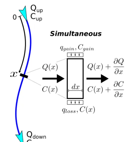
Following this rationale, this paper presents a new method based on a different assumption for the spatial distribution of SGE as compared to the GL (max) and LG (min) meth-ods, namely that bothQgainandQlossoccur simultaneously and uniformly throughout the entire stream section. This new method is denoted as “SIM”. Equations requiring the same input data as the GL (max) and LG (min) methods are de-rived in Sect. 2.2 and length is integrated into the mass bal-ance equation (Fig. 3).

2.2 Derivation of the method for simultaneous gains

and losses

In this section, the fundamental equations of mass balance for the tracer and water flows will be applied on a control volume represented in Fig. 3 under the assumption of simultaneous and uniform gains and losses throughout the stream reach and stationarity in time in order to obtain the expressions predictingQgainandQlossas functions ofQup,Cup,Qdown, CdownandCgain. First, applying mass balance for discharge: Q(x)+qgaindx=Q(x)+

∂

Q(x)∂xdx+qlossdx, (11)

Simultaneous

Q

0

C

Q

C

Figure 3. A conceptual representation of the analytical formulation of the SIM method.

wherex is distance along the stream,Q(x)is the discharge at lengthx,qgain is the added discharge per unit length of stream, and qloss is the lost discharge per unit of length. Bothqgainandqlossare assumed constant for a given stream reach. In the one-dimensional and stationary case, we can write∂Q(x)_∂x dx= dQ. After rearranging and integrating from the beginning of the reach over an arbitrary length,

Q(x)

Z

Qup

dQ=

x

Z

0

qgain−qlossdx, (12)

which becomes

Q(x)=Qup+ qgain−qlossx. (13)

Then, applying mass balance for the tracer,

˙

m(x)+Cgainqgaindx

=

˙

m(x)+∂m(x)˙

∂x dx

+C(x)qlossdx, (14)

wherem(x)˙ is the mass flow at lengthx,C(x)is the con-centration at lengthx, andCgainis the concentration ofqgain.

˙

m(x)is defined asm(x)˙ =Q(x)·C(x). The inflowing con-centrationCgainis assumed constant for a given stream reach. Again, in the one-dimensional and stationary case we can write ∂m(x)_∂x˙ dx= dm˙. Taking into account the definition of

˙

m(x), we can writedm˙= d(C·Q) =Q·dC+C·dQ. Rear-ranging the equation we get

Substituting Eqs. (12) and (13) forQ(x)anddQrespectively in Eq. (15), and rearranging, yields

dC=Cgainqgaindx−C(x)

qgain−qlossdx+qlossdx Qup+ qgain−qlossx

. (16) Simplifying and integrating from the beginning of the reach over an arbitrary lengthx yields

C(x)

Z

Cup

dC C(x)−Cgain

=−qgain

x

Z

0

dx Qup+ qgain−qloss

x (17)

which becomes lnC(x)−Cgain

Cup−Cgain

=− qgain

qgain−qloss

lnQup+ qgain−qloss

x Qup

. (18) Evaluating Eq. (13) for x=L, where Lrepresents the total length of the stream reach, yields

qgain−qloss=

Qdown−Qup

L . (19)

Substituting Eq. (19) in Eq. (18) and evaluating for x=L

yields

lnCdown−Cgain

Cup−Cgain

=− qgain

Qdown−Qup

L

lnQdown

Qup

. (20)

CallingQgain=qgain·Land rearranging yields

Qgain,SIM= Qup−Qdown

lnhC_Cdown−Cgain

up−Cgain

i

lnhQdown

Qup

i . (21) If we substitute Eq. (2) forQgain,SIMin Eq. (21), the solution forQlossis

Qloss,SIM= Qup−Qdown

lnhQdown(Cdown−Cgain)

Qup(Cup−Cgain)

i

lnhQdown

Qup

i , (22) whereQgain,SIMandQloss,SIMare the SIM equations for the SGE into and out of the stream, respectively.

As with the previous methods, if we use an artificial tracer (e.g., bromide salt) we can safely assumeCgain≈0 and the resulting equations are as follows:

Qgain,SIM= Qup−Qdown

lnhCdown

Cup

i

lnhQdown

Qup

i (23)

and

Qloss,SIM= Qup−Qdown

lnhQdownCdown

QupCup

i

lnhQdown

Qup

i . (24)

Equations (21)–(24) are discontinuous when Qup=Qdown. Fortunately, this is a removable discontinuity and can be solved by applying L’Hôpital’s rule (Arfken and Weber, 2005). Applying L’Hôpital’s rule to Eq. (21) and differen-tiating forQupresults in the following:

Qgain,SIM=−Qup·ln _C

down−Cgain Cup−Cgain

. (25)

Equation (25) is the solution for the condition that

Qup=Qdownand applies to bothQgain,SIMandQloss,SIM as they will produce the same result in that situation. This is only a mathematical exception and should not be needed in practice asQup andQdown should not truly be equal when measured in the natural environment due to the natural het-erogeneity of streams and the inherent measurement error of the method to measure discharge.

Naturally occurring tracers (e.g., chloride salt) can also be applied to the SGE equations with additional information aboutCgain. As long as a quasi-steady-state condition applies and thatQgain>0, the only additional information to be col-lected would be theCup andCdownprior to the injection of the tracer. For the derivation, we can use any one of the three SGE methods (six possible equations) and they all will pro-duce the same final equation as the final equation is not re-liant on spatial distribution assumptions. For a more thorough derivation starting from the initial mass balance equations, refer to Appendix A. For simplicity, we will use theQgain,LG equation from Eq. (5). As the value ofQgain,LG will be the same before and after the tracer injection, we can make two versions of theQgain,LG before and after the tracer injection with a differentCup andCdown prior to the injection of the tracer and post injection of the tracer.

Qdown _C

down,prior−Cup,prior Cgain−Cup,prior

=Qdown

_C

down,post−Cup,post Cgain−Cup,post

(26) and with some rearrangement, we come to our final equation:

Cgain=

Cup,priorCdown,post−Cdown,priorCup,post Cup,prior−Cup,post−Cdown,prior+Cdown,post

, (27)

2720 M. Exner-Kittridge et al.: Stream to groundwater exchange models

SGE. If the difference between the Qup andQdownis very small, much tracer may be needed to accurately measure a concentration difference betweenCupandCdown. This issue will become more important with larger rivers as the pro-portion of the Qgain and Qloss to the Qup is substantially reduced.

It would also be possible to estimateCgain from ground-water piezometers adjacent to the bank of the stream. As the intent of our study was to determine integrated values over a stream reach rather than point values, we preferred to use Eq. (27) as it is an integrated value ofCgain.

The application of tracer methods to measure SGE in the field is typically performed by two different techniques: con-stant injection and slug injection. These two techniques have been well researched in the scientific community and will not be evaluated in this study (Wagner and Harvey, 1997; Payn et al., 2008). Both techniques can be used with the above SGE methods and provide very similar results. As slug injections cause the Cdown to not be in a steady state, Cdown must be continuously measured and integrated over the measurable period of time. A more thorough explana-tion can be found in Payn et al. (2008, 2009) and Covino et al. (2011). For simplicity, we will assume constant injec-tion with steady-state condiinjec-tions.

2.3 Evaluation methods

2.3.1 Analytics

All three SGE methods were broken down analytically to bet-ter understand the dynamics of the equations of the methods. We wanted to know what caused the differences in the re-sults of the three SGE methods and how these differences were related. The relative differences between the methods were accomplished by the ratio of one method’s equation to another both analytically and illustratively.

2.3.2 Numerical simulations

Perfect measurements or estimates of SGE are impossible using any existing method. Arbitrarily comparing results of different methods using field collected data will only indi-cate that the different methods produce different results, and it will not indicate if one method is more accurate than an-other. Consequently, we thought that it would be appropriate to simulate artificial streams with known SGE for compar-isons. With SGE perfectly known, we could effectively eval-uate the accuracy of the different methods.

We simulated the lateral inflows and outflows per unit length throughout a stream using an autoregressive inte-grated moving average (ARIMA) model performed using the arima.sim package in the R statistical computing environ-ment (R Developenviron-ment Core Team, 2011). The routine gen-erates a variety of artificial time series with both a random-ness and memory component. To represent a small stream,

the ARIMA model was designed to take a random discharge of between 1 and 5 L s−1as input discharge and a random input tracer concentration of between 20 and 150 mg L−1to represent practical tracer test concentrations.

In an attempt to create realistic simulations of the streams, we tuned the ARIMA model to have spatial flux dynamics based on studies using distributed temperature sensing (DTS) of groundwater inflows within streams (Lowry et al., 2007; Westhoff et al., 2007; Briggs et al., 2012; Mwakanyamale et al., 2012). The quantitative surrogate we used for the spa-tial flux dynamics was the average length that the fluxes would switch from inflow to outflow or vice versa within a stream reach. For example, if we simulate a stream with 1000 m total length and the fluxes in this stream oscillate be-tween inflows and outflows 10 times then the average length per switch would be 100 m. For our simulations, we used two different switch lengths of 100 and 200 m and total stream lengths of 1000 and 2000 m. The switch lengths had a strong linear relationship with the correlation lengths and resulted in correlation lengths of 40 and 70 m for the switch lengths of 100 and 200 m, respectively. Correlation length is commonly defined as the length at 1/eon the autocorrelation distribu-tion (Blöschl and Sivapalan, 1995).

We used stream lengths of 1000 and 2000 m in the sim-ulations for two main reasons. First, the stream lengths of 1000 and 2000 m scale well with the switching lengths of 100 and 200 m and could easily be converted to nondimen-sional values if needed. Second, the lengths fit within prac-tical tracer test lengths that have been performed in the past to determine stream to groundwater exchange, albeit towards the upper end (Covino et al., 2011). In practice, the appropri-ate stream lengths will be dependent on the discharge in the stream, the available mass of tracer, and the sensitivity and accuracy of the laboratory analytical methods.

The ARIMA model allowed us to create 5000 simulations of stream fluxes within a hypothetical stream. We ran four series of 5000 simulations. Series A had a 1000 m stream length and a 100 m average switch length, series B had a 1000 m and a 200 m average switch length, series C had a 2000 m and a 100 m average switch length, and series D had a 2000 m and a 200 m average switch length. The spatial dis-cretization of the model was 1 m for all series and simula-tions. These four series of simulations were to test the effects of both length and intermittency on the stream flux methods. Without loss of generality, we definedCgain= 0 for the simu-lations, which would be equivalent to the use of an artificial tracer (e.g., bromide salt) for the tracer test.

The second assumption was that both QgainandQloss can-not occur simultaneously at one point. In this assumption, only one vector of SGE was created that could oscillate be-tween Qgain andQloss. We decided to omit the option for simultaneity ofQgainandQlossthroughout the stream as this assumption coincided too closely with the assumption in the SIM method. To ensure a more rigorous evaluation against the SIM method, we decided to omit the ARIMA model as-sumption of simultaneity and only use the nonsimultaneity assumption for the simulations.

We attempted to simulate the stream with realistic dynam-ics of SGE, but we also tried to keep the model complexity as simple as possible. Although we did attempt to cover a wide range of SGE conditions when creating the many simu-lations, we undoubtedly did not cover all possible SGE con-ditions that could exist in nature. Realistically, the scientific community does not even know the full range of possibilities for natural SGE. We have also likely created simulations of SGE that do not exist in nature. Both issues are unavoidable when creating hydrologic simulations, particularly with the stochastic generation approach used in this paper. The hope is that the flux distributions of the simulations do closely rep-resent reality for the purpose of our evaluation.

The statistical evaluation consisted of several methods and procedures. First, we took all of the simulated scenarios (5000 in our case) within an individual series and averaged the inflows and outflows for each simulation. This gave us an average inflow to the stream and outflow from the stream over the entire length of the stream for each scenario and served as our "true" values of the fluxes that the other SGE methods would be compared to. Next, we calculated the SGE of each scenario using the three SGE methods from the start-ing and end values of the scenarios. We did not include ad-ditional randomness in the input values for the SGE meth-ods, which would equate to measurement error. This is due to the large variety of measurement devices and techniques that could be used in a tracer test, and each device and tech-nique would have different measurement errors associated with them. Additionally, we calculated the net flux (we will call “Net”) simply by subtractingQupfromQdown. We con-sidered the Net as the upper error benchmark for the evalua-tion as the estimaevalua-tion of Net requires less informaevalua-tion and should therefore perform worse than the other three SGE methods that require more information.

Once the SGE was calculated for all of the methods to be evaluated, we used as a performance measure the absolute normalized error for method m and for each simulation i, defined as

ε_im=

Qm_est,i−Qtrue,i

Qtrue,i

i=1, . . . ,5000, (28) whereQm_est,i is the estimated gross gain or loss value from the SGE methodmand simulationiandQtrue,iis the average

flux from the ARIMA model at simulationi. The results of

ε_im are two vectors (one for gross gains and one for gross

losses) for each of the four methods. Each vector contains 5000 elements, one for each scenario. To make an overall evaluation for each method, we simply took an average of all of the scenarios in each series for both vectors of gains and losses:

εm=1

n

n

X

i=1

ε_im, (29)

whereεmis the mean absolute normalized error (MANE) for each methodm (either flux leaving the stream or entering the stream) andn is the total number of scenarios in each series (5000). This is a compound measure of relative bias and accuracy.

We also used the normalized root-mean-square error (NRMSE) as a supplement to the MANE:

NRMSE=

s 1

n n

P

i=1

Qm_est,i−Qtrue,i

2

1

n n

P

i=1

Qtrue,i

. (30)

The use of the NRMSE to supplement the MANE is to pro-vide a higher weight to larger errors and scatter as compared to the MANE.

In addition to calculating theεmfor all of the SGE meth-ods, we compared theεm_i within each of the SGE methods to determine how frequently one method outperformed another:

rm1,m2= 1

n

n

X

i=1

1 ifεm1_i < εm2_i

0 ifεm1_i ≥ ε_im2, (31)

whererm1,m2 is the frequency of m1 SGE method outper-forming m2 SGE method.

Onceε_imandεmwere estimated, we wanted to determine the causes of the errors in the individual methods. This was accomplished through a correlation ofεm_i to various combi-nations of the input parameters.

3 Results

3.1 Analytics

When there is 0 flux of eitherQgainorQlossall three equa-tions produce the same results. For example, ifQloss= 0 then Eq. (2) becomes

Qdown=Qup+Qgain. (32)

2722 M. Exner-Kittridge et al.: Stream to groundwater exchange models

2 4 6

8

1 2 3 4 5 6 7 8 9 10

0.1

0.3

1

3

10

Qup Qdo

wn

GL

(

m

a

x

)

LG

(

m

in

)

Stream Loss (Qloss)

1 2 3 4 5 6 7 8 9 10 1 3

10 30

0.1

0.3

1

3

10

Stream Gain (Qgain)

1.2 _1.4 1.6

1.8 2

2.2

2.4 2.6

2.8 3

3.2

1 2 3 4 5 6 7 8 9 10

0.1

0.3

1

3

10

Qup Qdo

wn

S

IM

LG

(

m

in

)

1 2 3

4 5 6 7

1 2 3 4 5 6 7 8 9 10

0.1

0.3

1

3

10

1.5

2

2.5 3 3.5 4 4.5

1 2 3 4 5 6 7 8 9 10

0.1

0.3

1

3

10

Qup Qdo

wn

GL

(

m

a

x

)

S

IM

Cup Cdown

1 2

3 4 5

6 7 8

1 2 3 4 5 6 7 8 9 10

0.1

0.3

1

3

10

CupCdown

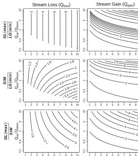
Figure 4. Relative comparisons between the different methods due to changes in the input ratios. The rows are the ratios of two of the SGE

methods and the columns are the results forQlossandQgain. In the two graphs in the middle panels, for example, if the ratio of the input

parametersCupandCdownis 5 and the ratio of the input parametersQupandQdownis 1 then the SIM method will result inQlossandQgain

being approximately 2 times larger than the LG (min) method. Theyaxes of_QQup

downis on a logarithmic scale to ensure equal space weighting

on the plot forQupandQdown. Thexaxes are plotted from 1 to 10 asCup≥Cdown.

Although somewhat obvious, if all of the assumptions are met for any of the SGE methods then the method will per-fectly reproduce reality. For example, if there is only inflow to the stream from 1–100 m followed by only flow out of the stream from 101–1000 m then the GL (max) equation will es-timate both fluxes perfectly.

If Qgain>0 and if Cgain< Cup then Cdown< Cup. Simi-larly, if Cgain> Cup then Cdown> Cup. This indicates that Cup andCdown are the concentration end points within the stream reach. As formulated in Eqs. (7)–(10), the LG (min) and GL (max) equations are divided by the end-point concen-trations of the stream and will therefore represent the mini-mum and maximini-mum values of fluxes within a stream reach. The LG (min) equations will always produce the minimum flux values, while the GL (max) equations will always pro-duce the maximum flux values. Consequently, as LG (min) and GL (max) have the minimum and maximum flux values, the flux values for the SIM equations must be somewhere in between the two.

The GL (max) and LG (min) methods are very similar, and subsequently can be compared quite easily. Dividing the in-flow and outin-flow equations for the two methods can show the rate of increase of one method over the other:

Qloss,GL Qloss,LG

= Cup

Cdown

(33) and

Qgain,GL Qgain,LG

= QupCup

QdownCdown

. (34)

For bothQlossandQgain, GL (max) grows from LG (min) at a rate proportional to the concentration ratio, and additionally

Qgaingrows with load ratio. AsQlossandQgainincrease in a stream reach,Qdownwill change andCdownwill decrease. In the case of a lowerCdowncaused by higher SGE, the ratio between the results of GL (max) and LG (min) grows larger (Fig. 4).

Flow (l/s)

Qloss

0 1 2 3 4

0.0

0.2

0.4

0.6

Flow (l/s)

Qup

0 1 2 3 4 5

0.00

0.10

0.20

Concentration (mg/l)

Cup

0 50 100 150

0.000

0.004

0.008

Flow (l/s)

Qgain

0 1 2 3 4

0.0

0.2

0.4

0.6

Flow (l/s)

Qdo

wn

0 2 4 6 8

0.00

0.10

0.20

Concentration (mg/l)

Cdo

wn

0 50 100 150

0.000

0.005

0.010

0.015

Flow (l/s)

Qnet

(Q

gain

−

Qloss

)

−4 −2 0 2 4

0.0

0.1

0.2

0.3

−

Qup Qdo

wn

0 1 2 3 4 5

0.0

0.4

0.8

1.2

−

Cup Cdo

wn

1 2 3 4 5 6 7 8

0.0

0.2

0.4

0.6

0.8

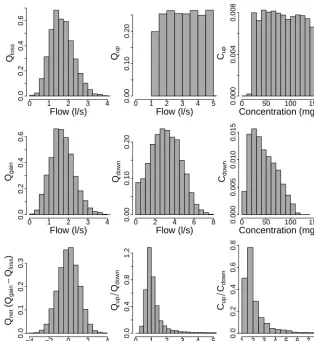
Figure 5. The major input and output parameter density distributions of the ARIMA numerical model for series A (1000 m with 100 m average switch length).

plotted together with axes of concentration and discharge ra-tios (Fig. 4). As shown analytically in Eqs. (33) and (34), the ratio of GL (max) to LG (min) is insensitive to discharge for Qlossand sensitive to both discharge and concentration for Qgain. The ratios of SIM to the other methods illustrate the nonlinearity of the method. The methods’ ratios forQgain show a surprising similarity in the distribution of the contours even though the magnitudes are different.

3.2 Numerical simulations

Figure 5 presents the major input and output parameter den-sity distributions created by the ARIMA simulations for the inflow and outflow profiles. The parameter distributions for

Qloss,Qgain, andQnetclosely follow a normal distribution. As defined in the model,QupandCupare equally distributed between 1–5 L s−1and 20–50 mg L−1, respectively.

The results of the numerical simulations are presented in Tables 1, 2, and 3. Plots of the estimated gains and losses to the actual gains and losses for each of the methods for series A are illustrated in Fig. 6. The plots for the other scenarios have similar patterns only with a greater or lesser degree of