www.hydrol-earth-syst-sci.net/19/4689/2015/ doi:10.5194/hess-19-4689-2015
© Author(s) 2015. CC Attribution 3.0 License.
Defining high-flow seasons using temporal streamflow
patterns from a global model
D. Lee1, P. Ward2, and P. Block1
1University of Wisconsin – Madison, Madison, Wisconsin, USA
2Institute for Environmental Studies (IVM), VU University Amsterdam, the Netherlands
Correspondence to: P. Block ([email protected])
Received: 8 April 2015 – Published in Hydrol. Earth Syst. Sci. Discuss.: 30 April 2015 Revised: 6 November 2015 – Accepted: 9 November 2015 – Published: 27 November 2015
Abstract. Globally, flood catastrophes lead all natural haz-ards in terms of impacts on society, causing billions of dol-lars of damages annually. Here, a novel approach to defining high-flow seasons (3-month) globally is presented by identi-fying temporal patterns of streamflow. The main high-flow season is identified using a volume-based threshold tech-nique and the PCR-GLOBWB model. In comparison with observations, 40 % (50 %) of locations at a station (sub-basin) scale have identical peak months and 81 % (89 %) are within 1 month, indicating fair agreement between modeled and observed high-flow seasons. Minor high-flow seasons are also defined for bi-modal flow regimes. Identified major and minor high-flow seasons together are found to well represent actual flood records from the Dartmouth Flood Observatory, further substantiating the model’s ability to reproduce the appropriate high-flow season. These high-spatial-resolution high-flow seasons and associated performance metrics allow for an improved understanding of temporal characterization of streamflow and flood potential, causation, and manage-ment. This is especially attractive for regions with limited observations and/or little capacity to develop early warning flood systems.
1 Introduction
Flood disasters rank as one of the most destructive natu-ral hazards in terms of economic damage, causing billions of dollars of damage each year (Munich Re, 2012). These flood damages have risen starkly over the past half-century given the rapid increase in global exposure (Bouwer, 2011; UNISDR, 2011; Visser et al., 2014). To specifically address
flood disasters from a global perspective, understanding of global-scale flood processes and streamflow variability is im-portant (Dettinger and Diaz, 2000; Ward et al., 2014). In re-cent decades, studies have investigated global-scale stream-flow characteristics using observed streamstream-flow from around the world (Beck et al., 2013; McMahon, 1992; McMahon et al., 2007; Peel et al., 2001, 2004; Poff et al., 2006; Probst and Tardy, 1987) and modeled streamflow from global hydrolog-ical models (Beck et al., 2015; van Dijk et al., 2013; Mc-Cabe and Wolock, 2008; Milly et al., 2005; Ward et al., 2013, 2014) to investigate ungauged and poorly gauged basins (Fekete and Vörösmarty, 2007). Despite this broad attention to annual streamflow and its connections to global climate processes and precursors, there has been relatively little at-tention paid to the intra-annual timing of streamflow, empha-sizing the need for analysis of seasonal streamflow patterns to further improve understanding of large-scale hydrology and atmospheric behaviors in the main (flood) streamflow sea-son globally (Dettinger and Diaz, 2000). Moreover, better assessment of streamflow timing and seasonality is impor-tant for addressing frequency and trend analyses, flood pro-tection and preparedness, climate-related changes, and other hydrological applications that possess important sub-annual characteristics (Burn and Arnell, 1993; Burn and Hag Elnur, 2002; Cunderlik and Ouarda, 2009; Hodgkins et al., 2003). This motivates further investigation of intra-annual temporal streamflow patterns globally.
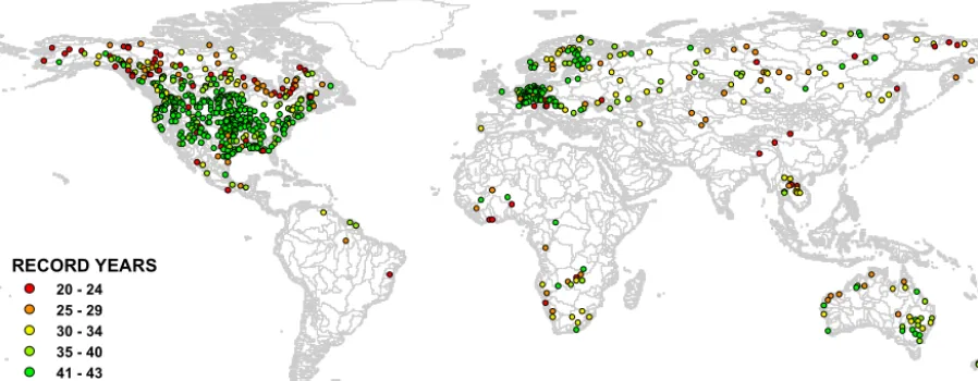
RECORD YEARS
[image:2.612.75.524.69.244.2]20 - 24 25 - 29 30 - 34 35 - 40 41 - 43
Figure 1. Location of 691 selected GRDC stations with the corresponding number of years per station. Background polygons are world sub-basins based on 300drainage direction maps (Döll and Lehner, 2002) with separation of large basins (Ward et al., 2014).
present one of the first maps providing a global classifica-tion. Burn and Arnell (1993) aggregate 200 streamflow sta-tions into 44 similar climatic regions and subsequently com-bine these into 13 groups using hierarchical clustering based on similarity of the annual maximum flow index, providing spatial and temporal coincidences of flood response. Det-tinger and Diaz (2000) aggregate 1345 sites into 10 clusters based on seasonality using climatological fractional monthly flows (CFMFs) to identify peak months and linkages with large-scale climate drivers.
In general, these studies define high streamflow or flood seasons subjectively based on the relationship between dom-inant streamflow amplitude patterns and large-scale climate drivers/patterns, and delineate large-scale homogeneous re-gions correspondingly. Defining high-flow season timing is essentially a bi-product of these analyses, and may be prob-lematic due to varying seasonal patterns (e.g., bi-modal dis-tribution, constant or low-flow areas, etc.) not captured at the large-scale delineation. There is also typically no distinc-tion between minor and high-flow seasons. In some cases, these minor seasons (e.g., resulting from bi-modal precipita-tion distribuprecipita-tion) can produce high-flow or flood condiprecipita-tions, and are thus of interest to identify. Here we identify high-flow seasons by capturing annual peak timing using a volumetric technique at the cell and sub-basin scale, presenting an ap-proach focused on streamflow temporal patterns rather than pattern of amplitude. The new measure of peak month (PM) and high-flow season (HS) coupled with the model grid scale provides much higher-resolution peak timings globally than previously presented (often at large basin scale or subcon-tinental scale). The performance measure introduced here, which is the percentage of annual maximum flow (PAMF), is also a new contribution relating the model’s ability to cap-ture high-flow season timing. These advantages are also help-ful for identifying less-dominant but important seasons
(mi-nor high-flow seasons) that possess similar characteristics to the high-flow season (e.g., a bi-modal annual cycle), an-other unique contribution of this work. This leads to better temporal characterization and understanding of flood poten-tial, causation, and management, particularly in ungauged or limited-gauged basins.
2 Data description 2.1 Streamflow stations
Daily streamflow observations utilized in this study are from the Global Runoff Data Centre (GRDC, 2007), specifically those stations located along the global hydrology model’s drainage network. Since station records that are missing even short periods may affect how a high-flow season is defined, we have excluded years with any daily missing values. In this study, a minimum of 20 hydrological years is required for a station to be retained, leaving 691 stations from all con-tinents except Antarctica, with upstream basin areas rang-ing from 9539 to 4 680 000 km2 and periods of record be-tween 20 and 43 years across 1958–2000 (Fig. 1). Although this criterion is admittedly quite strict (no missing 20-year daily data), including stations with missing records does not add a significant number. These stations are mostly located on large rivers; the annual streamflow of 75 % of stations is larger than 100 m3s−1, 35 % of stations are larger than 500 m3s−1, 20 % of stations are larger than 1000 m3s−1, and 5 % of stations are larger than 5000 m3s−1.
2.2 PCR-GLOBWB
Wa-ter Balance), a global hydrological model with a 0.5◦×0.5◦
resolution (Van Beek and Bierkens, 2009; Van Beek et al., 2011). Although the PCR-GLOBWB model is not cali-brated, and simulations may contain biases and uncertainty at course spatial resolution, the long time series of stream-flow provided globally has been deemed sufficient to esti-mate long-term flow characteristics with spatial consistency (Winsemius et al., 2013). Additionally, this model has been validated in previous studies in terms of streamflow (Van Beek et al., 2011) and terrestrial water storage (Wada et al., 2011) at stations along major rivers in the world. The model’s extreme discharges are also evaluated by Ward et al. (2013) with fair to good performance at stations with large drainage area (≥125 000 km2), corresponding to 24 % of GRDC sta-tions used in this study, excepting overestimation in several arid regions. Note that for the simulations used in this study, the maximum storage within the river channel is based on geomorphological laws that do not account for existing flood protection measures such as dikes and levees.
For the simulations used in this study, the PCR-GLOBWB model was forced with daily meteorological data from the WATCH (Water and Global Change) project (Weedon et al., 2011), namely precipitation, temperature, and global radi-ation data. These data are available at the same resolution as the hydrological model (0.5◦×0.5◦). The WATCH forc-ing data were originally derived from the ERA-40 reanalysis product (Uppala et al., 2005), and were subjected to a num-ber of corrections including elevation, precipitation gauges, timescale adjustments of daily values to reflect monthly ob-servations, and varying atmospheric aerosol loading. It is possible that this may have some minor effect on streamflow simulation, likely providing more realistic outcomes. Full de-tails of corrections are described in Weedon et al. (2011).
3 Defining high-flow seasons
To identify spatial and temporal patterns of dominant stream-flow uniformly, we design a fixed time window for represent-ing flow seasons globally. Here we define major high-flow seasons as the 3-month period most likely to contain dominant streamflow and the annual maximum flow. The central month is referred to as the peak month (PM) and the full 3-month period is referred to as the high-flow sea-son (HS). Specifically, we define PM first, and then define HS as the period also containing the month before and after the PM. This approach is performed for both observed (station) and simulated (model) streamflow to gauge performance.
3.1 Methodology for defining grid-cell-scale high-flow seasons
In the last few decades, a number of studies have investigated the timing of peak flows in the context of analyzing flood sea-sonality, frequency and trends. Generally, two main
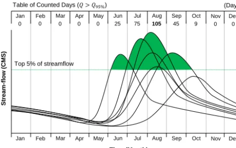
Top 5% of streamflow
Table of Counted Days (𝑄 > 𝑄95%) (Days)
S
tream
-f
lo
w
(
C
M
S
)
Time (Month)
Jan Feb Mar Apr May Jun Jul Aug Sep Oct Nov Dec
0 0 0 0 0 25 75 105 45 9 0 0
Jan Feb Mar Apr May Jun Jul Aug Sep Oct Nov Dec
Figure 2. Seven years of synthetic streamflow data. The dotted line represents the 5 % streamflow threshold. Numbers indicates the to-tal days above the threshold for each month.
days surpassing the 5 % threshold is listed for each month. In this example, August has the largest number of days over the threshold (105 days); thus, August is defined as PM and July–September is defined as HS.
To evaluate the defined HS objectively, by evaluating the number of annual maximum flows captured, we develop a simple evaluating statistic called the percentage of annual maximum flow (PAMF). PAMF is computed as shown in Eq. (1):
PAMF(i)=
i+1
P
j=i−1
nAMF(j )
12
P
k=1
nAMF(k)
, 1≤i≤12, (1)
where nAMF(i) denotes the number of annual maximum flows that occur in monthiacross the full record. In Eq. (1), wheniis 1 (January),i−1 in the summation is 12 (Decem-ber), and wheniis 12 (December),i+1 is 1 (January). Here the PAMF provides the percentage of annual maximum flows occurring in the defined HS across the evaluation period. The PAMF is relatively simple, yet provides a clear indication of how well the PM selected represents the occurrence of an-nual peaks across the time series. For example, a high PAMF indicates that the HS is highly likely to contain the annual maximum flood each year. In contrast, a low PAMF indi-cates that the timing of the annual maximum flow is more likely to vary temporally, and may be a result of bimodal sea-sonality, consistently high or low streamflow throughout the year, streamflow regulated by infrastructure or natural vari-ation. In this study, we subjectively classify HS PAMF val-ues as high (80–100 %), moderate (60–80 %), low (40–60 %) and poor (0–40 %). The PAMF is calculated for both the ob-served streamflow at the 691 selected GRDC stations and the simulated streamflow at the associated 691 grid locations.
The VBT technique is compared with the common volume-based technique and POT technique to gauge
per-formance. Four volume-based durations, namely V01 %, V03 %, V05 % and V10 %, and three POT techniques aver-aging 1, 2, and 3 peaks per year (POT1, POT2 and POT3, respectively), are selected. For the V01 % technique, the HS is simply centered on the PM containing the largest num-ber of occurrences of the top 1 % of annual streamflow vol-ume across the total years available. The V03 %, V05 % and V10 % techniques are similar to the V01 % approach, respec-tively using 3, 5 and 10 % of annual streamflow volume. Comparatively, techniques with a shorter time component (1–3 % of annual volume) favor identifying the PM by peak timing, since the top 1–4 days of streamflow tend be located near the peak, while techniques with longer time components (5–10 % of annual volume) favor identifying the PM based on duration and peak volume, since the top 19–33 days of streamflow tend to be located near the volumetric centroid of the hydrograph, rather than the peak, if they differ. The VBT technique is an attempt to bridge these two criteria. For the POT techniques, independence criteria are applied to avoid counting multiple peaks from the same event (Institute of Hy-drology, 1999). For example, two peaks must be separated by at least 3 times the average rising time to peak, and minimum flow between two peaks must be less than two-thirds of the higher one of the two peaks. More details of independence criteria are described in Lang et al. (1999).
An analysis examining sensitivity of selected threshold levels to the VBT technique is also undertaken. Performances of thresholds representing 1, 3, 5 and 10 % exceedance across the entire period of record, named VBT1 %, VBT3 %, VBT5 % and VBT10 %, respectively, are compared.
cap-Table 1. Cross-correlations of peak month (PM) at locations where the PMs differ by at least one classification technique (this occurs at 61 % of stations and 54 % of associated grids).
Classification technique VBT1 % VBT3 % VBT5 % VBT10 % V01 % V03 % V05 % V10 % POT1 POT2 POT3
Observed
VBT1 % 1.00
VBT3 % 0.90 1.00
VBT5 % 0.85 0.94 1.00
VBT10 % 0.79 0.86 0.91 1.00
V01 % 0.82 0.82 0.82 0.81 1.00
V03 % 0.81 0.84 0.83 0.84 0.89 1.00
V05 % 0.81 0.85 0.86 0.85 0.86 0.92 1.00
V10 % 0.80 0.84 0.85 0.87 0.83 0.88 0.96 1.00
POT1 0.78 0.78 0.78 0.74 0.76 0.77 0.76 0.74 1.00
POT2 0.74 0.78 0.78 0.78 0.80 0.80 0.82 0.81 0.81 1.00
POT3 0.77 0.81 0.81 0.80 0.80 0.81 0.83 0.81 0.86 0.93 1.00
Simulated
VBT1 % 1.00
VBT3 % 0.87 1.00
VBT5 % 0.83 0.95 1.00
VBT10 % 0.80 0.88 0.90 1.00
V01 % 0.86 0.85 0.84 0.84 1.00
V03 % 0.87 0.86 0.85 0.83 0.92 1.00
V05 % 0.87 0.88 0.85 0.84 0.90 0.97 1.00
V10 % 0.82 0.87 0.86 0.85 0.83 0.89 0.92 1.00
POT1 0.80 0.83 0.83 0.81 0.83 0.86 0.86 0.82 1.00
POT2 0.78 0.81 0.80 0.79 0.79 0.83 0.83 0.82 0.92 1.00
[image:5.612.55.538.95.346.2]POT3 0.80 0.81 0.79 0.80 0.80 0.83 0.84 0.81 0.92 0.95 1.00
Table 2. Average PAMF of each classification technique for modeled and observed streamflow where stations have different PMs.
Section VBT1 % VBT3 % VBT5 % VBT10 % V01 % V03 % V05 % V10 % POT1 POT2 POT3
Observed 60.8 % 61.7 % 62.0 % 62.0 % 63.4 % 63.6 % 63.0 % 62.5 % 60.8 % 59.1 % 60.6 %
Simulated 63.5 % 64.5 % 64.7 % 63.5 % 65.1 % 64.8 % 64.9 % 64.1 % 63.1 % 60.3 % 61.9 %
Table 3. Percentage of stations according to the difference in PMs between modeled and observed streamflow at each classification technique.
Difference VBT1 % VBT3 % VBT5 % VBT10 % V01 % V03 % V05 % V10 % POT1 POT2 POT3
in PMs
Same 39 % 39 % 40 % 42 % 38 % 39 % 40 % 42 % 38 % 36 % 38 %
≤ ±1 month 80 % 81 % 81 % 80 % 78 % 79 % 79 % 79 % 75 % 75 % 77 %
≤ ±2 month 90 % 91 % 91 % 90 % 89 % 90 % 89 % 89 % 87 % 87 % 88 %
≤ ±3 month 94 % 95 % 95 % 95 % 94 % 95 % 95 % 95 % 93 % 93 % 94 %
ture annual peak flows on a year-by-year basis, whereas the POT and VBT record significant peaks across the full time series, and may not capture annual peaks in some years in which that peak is small relative to all peaks throughout the available record. Thus VBT tends to select PMs that con-tain the most significant peaks overall, and subsequently have the highest potential for capturing probable flood seasons for flood-prone basins, a desirable outcome for this study. To il-lustrate this in the context of the PAMF, if all years are ranked for each location based on the annual peak flow, and the top 50 % (half) are retained, the PAMF actually favors the VBT
approach, surpassing the volume-based approach by 5–6 % for PMs and 2–3 % for HSs.
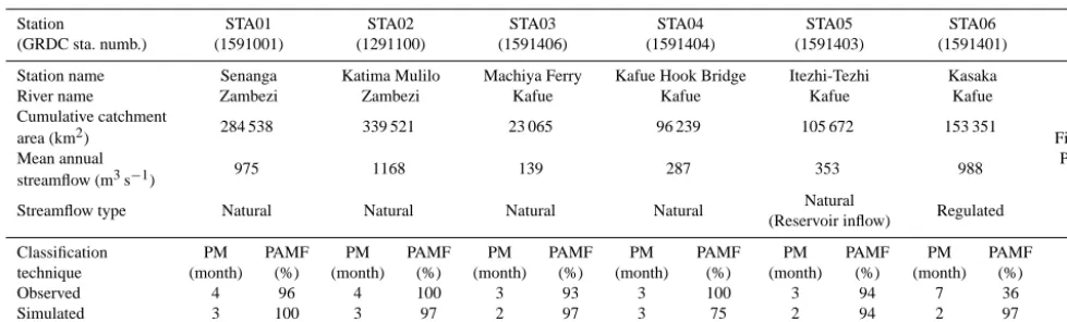
[image:5.612.58.541.388.429.2] [image:5.612.54.541.468.546.2]con-Table 4. Comparison of peak month (PM) for flooding and calculatedPAMFat six GRDC stations in the Zambezi River basin.
Station STA01 STA02 STA03 STA04 STA05 STA06
(GRDC sta. numb.) (1591001) (1291100) (1591406) (1591404) (1591403) (1591401)
Station name Senanga Katima Mulilo Machiya Ferry Kafue Hook Bridge Itezhi-Tezhi Kasaka
River name Zambezi Zambezi Kafue Kafue Kafue Kafue
Cumulative catchment
284 538 339 521 23 065 96 239 105 672 153 351
area (km2) Final
Mean annual
975 1168 139 287 353 988 PM
streamflow (m3s−1)
Streamflow type Natural Natural Natural Natural Natural Regulated
(Reservoir inflow)
Classification PM PAMF PM PAMF PM PAMF PM PAMF PM PAMF PM PAMF
technique (month) (%) (month) (%) (month) (%) (month) (%) (month) (%) (month) (%)
Observed 4 96 4 100 3 93 3 100 3 94 7 36 3
Simulated 3 100 3 97 2 97 3 75 2 94 2 97 2
sidering the 5 % threshold; thus, the remainder of the analysis is carried out utilizing the VBT5 % technique only.
3.2 Methodology for defining sub-basin-scale high-flow seasons
In addition to evaluating the HS at the 691 grid cells based on model outputs, the PM and HS can also be de-fined at the sub-basin scale globally where observations are present. Previous studies have investigated flood seasonal-ity as it relates to basin characteristics; for example, basins are delineated/regionalized and grouped according to sim-ilarity/dissimilarity of streamflow seasonality (Burn, 1997; Cunderlik et al., 2004a), or conversely, flood seasonality is occasionally used to assess the hydrological homogeneity of a group of regions (Cunderlik and Burn, 2002; Cunderlik et al., 2004b); thus, evaluating at the sub-basin scale is war-ranted.
While defining a single PM for a large-scale basin may be convenient, it may be difficult to justify given the potentially long travel times and varying climate, topography, vegeta-tion, etc. Additionally, infrastructure may be present to reg-ulate flow for flood control, water supply, irrigation, recre-ation, navigrecre-ation, and hydropower (WCD, 2000), causing managed and natural flow regimes to differ drastically. This becomes important, as globally more than 33 000 records of large dams and reservoirs are listed (ICOLD, 2009), with geo-referencing available for 6862 of them (Lehner et al., 2011). Nearly 50 % of large rivers with average streamflow in excess of 1000 m3s−1are significantly modulated by dams (Lehner et al., 2011), often significantly attenuating flow hy-drographs and flood volumes (20 % of GRDC stations fall into this category). The PAMF, as previously defined, can aid in identifying stations affected by upstream reservoirs through low PAMF values. This is applied with the assump-tion that reservoir flood control disperses the annual maxi-mum flows across months rather concentrated within a few months (e.g., akin to natural flow). In this study, we used the global sub-basins from the 300global drainage direction
map (DDM30) data set (Döll and Lehner, 2002) with separa-tion of large basins (Ward et al., 2014).
To define a sub-basin’s PM, the maximum PAMF and as-sociated PM for each station within the sub-basin are consid-ered according to the following:
– if multiple stations exist within the sub-basin, the PM is defined as the PM occurring for the largest number of stations;
– if there is a tie between months, their average PAMF values are compared, and the month having the higher average PAMF is defined as the PM;
– if there is a tie between months and equivalent average PAMF values, the month having the higher average an-nual streamflow is defined as the PM.
[image:6.612.51.541.84.232.2]Figure 3. Map of the Zambezi River basin; the solid black line delineates the basin and the green points are the six GRDC sta-tions (STA01-06), with STA06 downstream of the Itezhi-Tezhi dam (STA05).
In contrast, the model-based simulated streamflow pro-duces a high PAMF at STA06 (97 %), as the Itezhi-Tezhi dam is not represented in the simulations used for this study, and subsequently does not account for modulated stream-flow. Across other stations, the PAMF is also high; however, an equal number of stations select February and March. In this case, February is selected as the final basin PM given its higher average PAMF value (96 % vs. 91 %).
By this approach, all 691 GRDC stations are grouped into 223 sub-basins to define the PM (Fig. 6); 58 % of sub-basins are defined by a single station, only 7.6 % (observations) and 8.1 % (model) of sub-basins have ties when defining PMs, and only one sub-basin has a tie between PMs and average PAMF values.
4 Verification of selected high-flow seasons
Model-based PMs are verified by comparing with observation-based PMs at station and sub-basin scales. Additionally, historic flood records from the Dartmouth Flood Observatory (DFO) are used to compare basin-level PMs to actual flooded areas spatially and temporally. Specif-ically, we apply the following information from DFO: start time, end time, duration and geographically estimated area at 3486 flood records across 1985–2008.
4.1 Observed versus modeled high-flow seasons Ideally the model-based and observed GRDC stations have fully or partially overlapping HS periods. If so, this builds confidence in interpreting HSs at locations where no served data are available. For comparing modeled PMs to ob-servations, the defined PMs and calculated PAMF are repre-sented globally at the station scale (Figs. 4–5) and sub-basin scale (Fig. 6) with temporal differences of PMs (modeled PM – observed PM). In the southeastern United States, GRDC
stations express relatively lower PAMF values for observa-tions (40–60 %) than model outputs (60–80 %), due to the high level of managed infrastructure. In the central–southern US and Europe, low PAMF values are computed for both ob-servations and modeled output (Fig. 5) with notable tempo-ral differences (Fig. 4c). For observations, this is attributable, at least in part, to reservoirs and dams along the Mississippi, Missouri and Danube rivers. Additionally, relatively constant streamflow patterns are identified in both observations and modeled output, consistent with previous studies reporting these flow regimes as uniform or perpetually wet (Burn and Arnell, 1993; Dettinger and Diaz, 2000; Haines et al., 1988). Minor high-flow seasons may also play a role. Model biases also affect PM selection; for northwestern North America, PMs for many points are defined on average 1 month ear-lier than with observations, producing moderate PAMF val-ues (60 % and higher). In northern Europe, especially south-ern Finland, this becomes much more pronounced, with large differences between PMs from observations and the model, on the order of 4 months (Figs. 4c, 6c, and 8a). In western and northern Australia, PMs are modeled 1 month later on average than observations, except for two occurrences in the west (5-month difference) due to both observed and modeled low-flow conditions. Such low-flow regimes are also appar-ent in southeastern Australia, causing large differences be-tween PMs (4–5 months). The differences in PMs bebe-tween observations and modeled outputs are also compared at the continental scale (Fig. 7). In North America, 38 % of stations and 51 % of sub-basins produce identical PMs, growing to 82 % of stations and 93 % of sub-basins when considering a±1 month temporal difference (e.g., HS; Fig. 7). In Asia 65 % of stations and 70 % of sub-basins have identical PMs, growing to 90 % of stations and 92 % of sub-basins with
±1 month temporal difference (Fig. 7). In central Russia, a large difference between PMs (±3 months) is attributable to reservoirs on the Yenisei and Angara rivers and model bias (Fig. 4c). In Africa, 48 % of stations and 60 % of sub-basins produce identical PMs (Fig. 7), 30 % of stations and 27 % of sub-basins are modeled 1 month earlier, and 7.4 % of stations and 6.7 % of sub-basins are modeled 1 month later than ob-servation (Fig. 7). In South America, with only five stations, 40 % have the same month, 40 % are modeled 1 month ear-lier, and 20 % of stations are modeled 2 months earlier than observations.
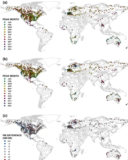
PM DIFFERENCE (SM-OB)
≤-4 -3 -2 -1 S +1 +2 +3 ≥+4
(c)
PEAK MONTH JAN FEB MAR APR MAY JUN JUL AUG SEP OCT NOV DEC
(b)
PEAK MONTH JAN FEB MAR APR MAY JUN JUL AUG SEP OCT NOV DEC
[image:8.612.94.508.68.585.2](a)
Figure 4. Peak month (PM) for flooding as defined by (a) 691 GRDC observation stations, (b) simulated streamflow at associated locations and (c) temporal difference in PM between observations and simulation (simulation–observation, in number of months; a negative (positive) value indicates that the simulated PM is earlier (later) than the observed PM).
9 % of locations and 8 % of sub-basins), a substantial num-ber are located downstream of reservoirs directly, such as STA06 in the Zambezi example (Table 4), or are low-flow (dry) or constant-flow locations, both producing exceedingly low PAMF values. Differences in PMs are not unexpected
PAMF 80-100% 60-80% 40-60% 20-40% 0-20%
(b)
PAMF 80-100% 60-80% 40-60% 20-40% 0-20%
[image:9.612.92.505.69.406.2](a)
Figure 5. Calculated percentage of annual maximum flow (PAMF) values for (a) 691 GRDC observation stations and (b) simulated stream-flow at associated locations, subjectively classified as high (80–100 %), moderate (60–80 %), low (40–60 %), and poor (0–40 %).
performs appropriately well in defining high-flow seasons globally at locations where observations are available.
This may be subsequently extended to defining PMs and PAMF at all grid cells (Fig. 8). Generally, low and poor PAMF values (0–60 %) indicate a naturally unstable annual maximum flow (no clear high-flow season), which occurs in cases of constant flow, low flow, bi-modal flow and regulated flow. All cases, except regulated flow, are simulated within the PCR-GLOBWB simulations used; thus, the cell-based PAMF values (Fig. 8b) can provide a sense of confidence for the defined PM (Fig. 8a). Examples of low-flow regions include the central United States and Australia, having low PAMF regional values (Fig. 8b). Bi-modal regions, such as much of eastern Africa and southern South America with their two rainy seasons, and constant-flow regions, such as Europe, also indicate low PAMF values (Fig. 8b). These flow regimes are further investigated as minor HS in Sect. 5.
4.2 Modeled high-flow seasons versus actual flood records
PM DIFFERENCE (SM-OB)
≤-4 -3 -2 -1 S +1 +2 +3 ≥+4
(c)
(b)
(a)
PEAK MONTH JAN FEB MAR APR MAY JUN JUL AUG SEP OCT NOV DEC
[image:10.612.99.503.65.568.2]PEAK MONTH JAN FEB MAR APR MAY JUN JUL AUG SEP OCT NOV DEC
Figure 6. Peak month (PM) for flooding by sub-basin as defined by (a) 691 GRDC observation stations, (b) simulated streamflow at asso-ciated sub-basins and (c) temporal difference in PM between observations and simulation (simulation–observation, in number of months; a negative (positive) value indicates that the simulated PM is earlier (later) than the observed PM).
Figs. 8a and 9), particularly when both the major and minor high-flow seasons are considered, further indicating merit in the ability of the proposed approach to identify the PM. Con-sistently, regions with high model-based PAMF (80–100 %), such as eastern South America, central Africa and central Asia, tend to agree well with DFO records, while poor or less than poor PAMF (0–60 %) regions, such as central North
0 10 20 30 40 50 60 70 80 90 100
Asia (10.4%)
Africa (3.9%)
North America (61.9%)
South America (0.7%)
Europe (18.1%)
Australia (4.9%)
Global (100%)
P
e
rc
e
nt
a
ge
of
s
ta
ti
ons
(%
)
0 10 20 30 40 50 60 70 80 90 100
Asia (16.6%)
Africa (6.7%)
North America (43.9%)
South America (2.3%)
Europe (20.6%)
Australia (9.9%)
Global (100%)
P
e
rc
e
nt
a
ge
of
s
ub
-b
asi
n
s
(%
)
[image:11.612.148.448.71.276.2]≤-3month -2month -1month Same +1month +2month ≥+3month
Figure 7. Percentage of stations (top panel) and sub-basins (bottom panel) according to the temporal difference of PM between observations and model outputs (SM–OB, number of months) in each continent.
(b)
STREAMFLOW Arid (<1cms)
PAMF
80-100% 60-80% 40-60% 20-40% 0-20%
(a)
PEAK MONTH
JAN FEB MAR APR MAY JUN JUL AUG SEP OCT NOV DEC
STREAMFLOW Arid (<1cms)
[image:11.612.95.508.338.679.2]MONTH
[image:12.612.85.511.69.231.2]JAN FEB MAR APR MAY JUN JUL AUG SEP OCT NOV DEC
Figure 9. Occurrence (start) months of 3486 events from the Global Active Archive of Large Flood Events from the Dartmouth Flood Observatory (DFO) over 1985–2008 (Brakenridge, 2011); polygons indicate the estimated spatial extent, colors represent the start month, with the most recent events layered on top.
5 Defining minor high-flow seasons
In some climatic regions, there is no one single, well-defined flood season. For example, eastern Africa has two rainy sea-sons, the major season from June to September and the minor season from January to April/May. These two seasons are in-duced by northward and southward shifts of the Inter-tropical Convergence Zone (ITCZ) (Seleshi and Zanke, 2004). This bi-modal eastern African pattern allows for potential flood-ing in either season. In Canada, as another example, the dom-inant spring snowmelt season (March–May) and fall rainy season (August–October) allow for flood occurrences in ei-ther period (Cunderlik and Ouarda, 2009).
Previous studies have investigated techniques to differen-tiate seasonality from uni-, bi- and multi-modal streamflow climatologies and evaluate trends in the timing and magni-tude of streamflow, including the POT method, directional statistics method, and relative flood frequency method (Cun-derlik and Ouarda, 2009; Cun(Cun-derlik et al., 2004a). These methods may perform well at the local (case-specific) scale to define minor high-flow seasons; however, applying them uniformly at the global scale can be problematic, given spatial heterogeneity. Additionally, even though bi-modal streamflow climatology may be detected, the magnitude of streamflow in the minor season may or may not be negligible in regards to flooding potential as compared with the major season.
To detect noteworthy minor high-flow seasons glob-ally, we classify streamflow regimes by climatology and monthly PAMF value, calculated using Eq. (1) at each month (Fig. 10). Classifications include unimodal, bimodal, con-stant, and low-flow. The unimodal streamflow climatology has high values of PAMF around the PM; the bi-modal classification is represented by two peaks of PAMF (and may therefore contain a minor season); both constant and
low-flow classifications represent low values of PAMF be-tween months. Distinguishing bebe-tween bi-modal and other classifications is nontrivial. For example, initial inspection of the constant streamflow classification (both climatology and monthly PAMF, Fig. 10c) could be mistaken for a non-dominant bi-modal distribution. We adopt the following cri-teria to differentiate bi-modal streamflow from uni-modal, constant, and low-flow conditions.
– The low-flow classification is defined for annual average streamflow less than 1 m3s−1.
– The major and minor PMs must be separated by at least 2 months in order to prevent an overlap of each HS (3 months).
– If there is a peak in the monthly PAMF values outside the major HS, it is regarded as a potential minor PM. If the sum of the major and potential minor PM’s PAMF is greater than 60 % (a minimum of 29 out of 43 annual maximums fall into one of the HS), the potential minor PM is confirmed as a minor PM; the major PM’s PAMF cannot exceed 80 %.
0 100 200 300
J F M A M J J A S O N D
S T R E A M FLOW ( 1 0 3C M S )
Amazon river, Brazil
0 20 40 60 80 100
J F M A M J J A S O N D
M O N TH LY PA M F (% )
Amazon river, Brazil
0 1000 2000 3000 4000
J F M A M J J A S O N D
STREA M FL O W (CM S)
Webi Shabeelie river, Somalia
0 20 40 60 80 100
J F M A M J J A S O N D
M O NTHLY PA M F (% )
Webi Shabeelie river, Somalia
0 200 400 600 800
J F M A M J J A S O N D
STREA M FL O W (CM S)
Lakekamu river, Papua New Guinea
0 20 40 60 80 100
J F M A M J J A S O N D
M O NTHLY PA M F (% )
Lakekamu river, Papua New Guinea
0.0 1.0 2.0 3.0
J F M A M J J A S O N D
STREA M FL O W (CM
S) Quequen Salado river, Argentina
0 20 40 60 80 100
J F M A M J J A S O N D
M O NTHLY PA M F (% )
Quequen Salado river, Argentina
(a)
(b)
(c)
[image:13.612.154.440.67.379.2](d)
Figure 10. Model-based streamflow climatology (left panels) and corresponding monthly PAMF (right panels). Types and locations are (a) uni-modal streamflow – at Bom Lugar, Amazon River, Brazil, (b) bimodal streamflow – at Saacow, Webi Shabeelie River, Somalia, (c) constant streamflow – at Terapo Mission, Lakekamu River, Papua New Guinea, and (d) low flow – at La Sortija, Quequen Salado River, Argentina.
constant or low streamflow (Fig. 10d). Minor HSs are sim-ilar to major HSs, containing the minor PM and the month before and after. Minor HSs are evident in the tropics and sub-tropics and are spatially consistent with bi-modal rain-fall regimes discovered by Wang (1994) (Fig. 11). Examples include eastern Africa (second rainy season in winter) and Canada (rainfall-dominated runoff in fall, both having high joint PAMF values (80–100 %). Additional examples include the major HS (NDJ) and minor HS (MAM) in central Africa consistent with the latitudinal movement of the ITCZ, intra-Americas’ major HS (ASON) and minor HS (AMJJ) (Chen and Taylor, 2002), and coastal regions of British Columbia in Canada and southern Alaska’s minor HS (SOND) due to win-tertime migration of the Aleutian low from the central North Pacific (Fig. 11). Distinct runoff process controlled by dif-ferent climate and hydrology systems can induce a bi-modal peak within a large-scale basin, such as the upstream sec-tions of the Yenisey and Lena river systems in Russia where the major HS (AMJ) is dominated by snowmelt and the mi-nor HS (JAS) is spurred on by the Asian monsoon. The same mechanism produces minor HSs around the extents of the Asian summer monsoon (90–100 % of the sum of PAMFs)
(Figs. 8b and 11). Moderate minor HSs include, for exam-ple, the southern United States’ (Texas and Oklahoma) bi-modal rainfall pattern (AMJ and SON) and the southwest-ern United States (Arizona), where the summertime major HS (JJA) is produced by the North American monsoon and the wintertime minor HS (DJF) is affected by the regional large-scale low-pressure system (Woodhouse, 1997). South-eastern Brazil’s summertime major HS (NDJF) and post-summer minor HS (AMJ) are dominated by formation and migration of the South Atlantic Convergence Zone (Herdies, 2002; Lima and Satyamurty, 2010). In central and eastern Europe, the major HS (FMAM) and minor HS (JJA) are de-fined as moderate (60–80 % of joint PAMF values for central Europe and 70–90 % for eastern Europe), indicating that a minor HS is not overly pronounced; for northeastern Europe the major HS (MAM) and minor HS (NDJ) contain high joint PAMF values (80–100 %).
(b)
STREAMFLOW
Arid (<1cms)
30N
30S EQ
JOINT PAMF
90-100% 80-90% 70-80% 60-70% 50-60%
(a)
STREAMFLOW
Arid (<1cms)
30N
30S EQ
PEAK MONTH
JAN FEB MAR APR MAY JUN JUL AUG SEP OCT NOV DEC
Figure 11. (a) Minor peak month (PM) for flooding as defined at detected grid cells and (b) joint PAMFs of major and minor PMs at corresponding cells; subjectively classified as high (80–100 %), moderate (60–80 %), and low (40–60 %).
between the HSs and monthly flood records (Fig. 12). Minor HSs with high PAMF values corresponding well to observed DFO flood records include eastern Africa (bi-modal stream-flow), the intra-Americas, and northern Asia; only a few re-ported flood records occur in the minor HSs at high latitudes.
6 Conclusions and discussion
In this study, a novel approach to defining high-flow sea-sons globally is presented by identifying temporal patterns of streamflow objectively. Simulations of daily streamflow from the PCR-GLOBWB model are evaluated to define the dominant and minor high-flow seasons globally. In order to consider both peak volume and peak timing, a volume-based threshold technique is applied to define the high-flow sea-son and is subsequently evaluated by the PAMF. To verify model-defined high-flow seasons, we compare with observa-tions at both station and sub-basin scales. As a result, 40 % of stations and 50 % of sub-basins have identical peak months
and 81 % of stations and 89 % of sub-basins are within 1 month, thus well capturing high-flow seasons. When con-sidering anthropogenic effects and bi-modal or perpetually wet/dry flow regions, these results indicate fair agreement between modeled and observed high-flow seasons. Regions expressing bi-modal streamflow climatology are also defined to illustrate potential for noteworthy secondary (minor) high-flow seasons. Model-defined major and minor high-high-flow sea-sons are additionally found to represent actual flood records from the Dartmouth Flood Observatory, further substantiat-ing the model’s ability to reproduce the appropriate high-flow season.
[image:14.612.79.521.67.422.2]find-DFO records Minor PM
Minor HS Major HS
[image:15.612.56.542.63.504.2]Major PM
Figure 12. Defined major HS and minor HS where joint PAMF is greater than 60 % (left panels); peak month of major and minor HSs (dense color) and pre- and post-month of major and minor HSs (light color). Monthly accumulated actual flood records (DFO) during 1958–2008 (right panels).
ings (e.g., Burn and Arnell, 1993; Dettinger and Diaz, 2000; Haines et al., 1988); however, this analysis goes further by not being constrained to large-scale patterns for seasonal def-inition (via clustering) and also providing a sense of the reli-ability of the defined high-flow seasons. Specifically, the de-fined PM (Fig. 8a) has extended Dettinger and Diaz (2000)’s peak months by focusing on basin- and grid-scale stream-flow volumes and providing likelihood type maps using the PMAF metric developed here (e.g., Fig. 8b) to represent the reliability of the defined PM. This can provide a clear sense of whether the identified high-flow season is pronounced or vague. The identification of minor high-flow seasons and
de-ciphering bi-modal from constant streamflow regimes is an-other notable contribution of this study; minor seasons have not been well identified in previous studies. These identified high-flow seasons are also consistent with DFO flood records both spatially and temporally, further substantiating their ap-propriateness.
in-dicate relatively positive performance overall, regional per-formance varies spatially. This is advantageous for many reasons, including hydrologic assessment in ungauged and poorly gauged basins and also for investigating flood sea-son timing within large basins having diverse physical pro-cesses, for example, how the PM may shift along long rivers (e.g., Congo River) or basins with both snowmelt and rain-dominated processes. These spatially heterogeneous high-flow seasons at high resolution have the potential to charac-terize streamflow regimes better than previous studies (e.g., Dettinger and Diaz, 2000; Haines et al., 1988). Additional analysis to include upstream management and regulations is required to further classify global streamflow regimes and major high-flow seasons (or the elimination of them) for spe-cific sub-basin-level hydrologic applications.
Acknowledgements. The first author was partially funded by a
grant from the University of Wisconsin – Madison. The second author was funded by a VENI grant from the Netherlands Organisa-tion for Scientific Research (NWO). We thank the editor and three anonymous reviewers for their valuable comments and suggestions.
Edited by: R. Woods
References
Beck, H. E., van Dijk, A. I. J. M., Miralles, D. G., de Jeu, R. A. M., Sampurno Bruijnzeel, L. A., McVicar, T. R., and Schellekens, J.: Global patterns in base flow index and recession based on streamflow observations from 3394 catchments, Water Resour. Res., 49, 7843–7863, doi:10.1002/2013WR013918, 2013. Beck, H. E., de Roo, A., and van Dijk, A. I. J. M.: Global Maps
of Streamflow Characteristics Based on Observations from Sev-eral Thousand Catchments, J. Hydrometeorol., 16, 1478–1501, doi:10.1175/JHM-D-14-0155.1, 2015.
Bouwer, L. M.: Have Disaster Losses Increased Due to Anthro-pogenic Climate Change?, B. Am. Meteorol. Soc., 92, 39–46, doi:10.1175/2010BAMS3092.1, 2011.
Brakenridge, G. R.: Global Active Archive of Large Flood Events, Dartmouth Flood Observatory, University of Colorado, available at: http://floodobservatory.colorado.edu/Archives/index.html, last access: 27 April 2015, 2011.
Burn, D. H.: Catchment similarity for regional flood frequency analysis using seasonality measures, J. Hydrol., 202, 212–230, doi:10.1016/S0022-1694(97)00068-1, 1997.
Burn, D. H.: Climatic influences on streamflow timing in the head-waters of the Mackenzie River Basin, J. Hydrol., 352, 225–238, doi:10.1016/j.jhydrol.2008.01.019, 2008.
Burn, D. H. and Arnell, N. W.: Synchronicity in global flood responses, J. Hydrol., 144, 381–404, doi:10.1016/0022-1694(93)90181-8, 1993.
Burn, D. H. and Hag Elnur, M. A.: Detection of hydrologic trends and variability, J. Hydrol., 255, 107–122, doi:10.1016/S0022-1694(01)00514-5, 2002.
Chen, A. A. and Taylor, M. A.: Investigating the link between early season Caribbean rainfall and the El Nino+1 year, Int. J. Clima-tol., 22, 87–106, doi:10.1002/joc.711, 2002.
Cunderlik, J. M. and Burn, D. H.: Local and Regional Trends in Monthly Maximum Flows in Southern British Columbia, Can. Water Resour. J., 27, 191–212, doi:10.4296/cwrj2702191, 2002. Cunderlik, J. M. and Ouarda, T. B. M. J.: Trends in the timing and magnitude of floods in Canada, J. Hydrol., 375, 471–480, doi:10.1016/j.jhydrol.2009.06.050, 2009.
Cunderlik, J. M., Ouarda, T. B. M. J., and Bobée, B.: Determination of flood seasonality from hydrological records/Détermination de la saisonnalité des crues à partir de séries hydrologiques, Hy-drolog. Sci. J., 49, 511–526, doi:10.1623/hysj.49.3.511.54351, 2004a.
Cunderlik, J. M., Ouarda, T. B. M. J., and Bobée, B.: On the ob-jective identification of flood seasons, Water Resour. Res., 40, W01520, doi:10.1029/2003WR002295, 2004b.
Dettinger, M. D. and Diaz, H. F.: Global Characteristics of Stream Flow Seasonality and Variability, J. Hydrometeorol., 1, 289–310, doi:10.1175/1525-7541(2000)001<0289:GCOSFS>2.0.CO;2, 2000.
Döll, P. and Lehner, B.: Validation of a new global 30-min drainage direction map, J. Hydrol., 258, 214–231, doi:10.1016/S0022-1694(01)00565-0, 2002.
Fekete, B. M. and Vörösmarty, C. J.: The current status of global river discharge monitoring and potential new technologies com-plementing traditional discharge measurements, Predict, in: Un-gauged Basins PUB Kick-off, IAHS Publ. no. 309, Proceedings PUB Kick-off Meet, held Novembember 2002, Brasil, 129–136, 2007.
GRDC – Global Runoff Data Centre: Major River Basins of the World/Global Runoff Data Centre, Federal Institute of Hydrol-ogy (BfG), Koblenz, Germany, available at: http://grdc.bafg.de, last acces: 27 April 2015, 2007.
Haines, A. T., Finlayson, B. L., and McMahon, T. A.: A global classification of river regimes, Appl. Geogr., 8, 255–272, doi:10.1016/0143-6228(88)90035-5, 1988.
Herdies, D. L.: Moisture budget of the bimodal pattern of the sum-mer circulation over South Asum-merica, J. Geophys. Res., 107, 8075, doi:10.1029/2001JD000997, 2002.
Hodgkins, G. A. and Dudley, R. W.: Changes in the timing of winter-spring streamflows in eastern North America, 1913–2002, Geophys. Res. Lett., 33, 1–5, doi:10.1029/2005GL025593, 2006. Hodgkins, G. A., Dudley, R. W., and Huntington, T. G.: Changes in the timing of high river flows in New England over the 20th Century, J. Hydrol., 278, 244–252, doi:10.1016/S0022-1694(03)00155-0, 2003.
ICOLD – International Commission on Large Dams: World Regis-ter of Dams, Version updates 1998–2009, ICOLD, Paris, avail-able at: www.icold-cigb.net, last acces: 27 April 2015, 2009. Institute of Hydrology: Flood Estimation Handbook, vol. 3, Institute
of Hydrology, Wallingford, UK, 1999.
Javelle, P., Ouarda, T. B. M. J., and Bobée, B.: Spring flood analysis using the flood-duration-frequency approach: application to the provinces of Quebec and Ontario, Canada, Hydrol. Process., 17, 3717–3736, doi:10.1002/hyp.1349, 2003.
Lehner, B., Liermann, C. R., Revenga, C., Vörösmarty, C., Fekete, B., Crouzet, P., Döll, P., Endejan, M., Frenken, K., Magome, J., Nilsson, C., Robertson, J. C., Rödel, R., Sindorf, N., and Wisser, D.: High-resolution mapping of the world’s reservoirs and dams for sustainable river-flow management, Front. Ecol. Environ., 9, 494–502, doi:10.1890/100125, 2011.
Lima, K. C. and Satyamurty, P.: Post-summer heavy rainfall events in Southeast Brazil associated with South Atlantic Convergence Zone, Atmos. Sci. Lett., 11, 13–20, doi:10.1002/asl.246, 2010. McCabe, G. J. and Wolock, D. M.: Joint Variability of Global
Runoff and Global Sea Surface Temperatures, J. Hydrometeo-rol., 9, 816–824, doi:10.1175/2008JHM943.1, 2008.
McMahon, T. A.: Global runoff: continental comparisons of annual flows and peak discharges, Catena Verlag, Cremlingen-Destedt, Germany, 1992.
McMahon, T. A., Vogel, R. M., Peel, M. C., and Pe-gram, G. G. S.: Global streamflows – Part 1: Charac-teristics of annual streamflows, J. Hydrol., 347, 243–259, doi:10.1016/j.jhydrol.2007.09.002, 2007.
Milly, P. C. D., Dunne, K. A., and Vecchia, A. V.: Global pattern of trends in streamflow and water availability in a changing climate, Nature, 438, 347–350, doi:10.1038/nature04312, 2005.
Munich Re: Topics Geo 2012 Issue, Natural
Catastro-phes 2011, Analyses, Assessments, Positions, Münchener Rückversicherungs-Gesellschaft, Munich, 2012.
Peel, M. C., McMahon, T. A., Finlayson, B. L., and Watson, F. G. R.: Identification and explanation of continental differences in the variability of annual runoff, J. Hydrol., 250, 224–240, doi:10.1016/S0022-1694(01)00438-3, 2001.
Peel, M. C., McMahon, T. A., and Finlayson, B. L.: Con-tinental differences in the variability of annual
runoff-update and reassessment, J. Hydrol., 295, 185–197,
doi:10.1016/j.jhydrol.2004.03.004, 2004.
Poff, N. L., Olden, J. D., Pepin, D. M., and Bledsoe, B. P.: Placing global stream flow variability in geographic and geomorphic con-texts, River Res. Appl., 22, 149–166, doi:10.1002/rra.902, 2006. Probst, J. L. and Tardy, Y.: Long range streamflow and world continental runoff fluctuations since the beginning of this cen-tury, J. Hydrol., 94, 289–311, doi:10.1016/0022-1694(87)90057-6, 1987.
Seleshi, Y. and Zanke, U.: Recent changes in rainfall and rainy days in Ethiopia, Int. J. Climatol., 24, 973–983, doi:10.1002/joc.1052, 2004.
Smith, R. L.: Threshold Methods for Sample Extremes, in: Statisti-cal Extremes and Applications, D. Reidel, Dordrecht, the Nether-lands, 621–638, 1984.
Smith, R. L.: Estimating Tails of Probability Distributions, Ann. Stat., 15, 1174–1207, doi:10.1214/aos/1176350499, 1987. Todorovic, P. and Zelenhasic, E.: A Stochastic Model for
Flood Analysis, Water Resour. Res., 6, 1641–1648,
doi:10.1029/WR006i006p01641, 1970.
UNISDR: Global Assessment Report on Disaster Risk Reduction (GAR 11) – Revealing Risk, Redefining Development, United Nations Office for Disaster Risk Reduction (UNISDR), Geneva, Switzerland, 2011.
Uppala, S. M., KÅllberg, P. W., Simmons, A. J., Andrae, U., Bech-told, V. D. C., Fiorino, M., Gibson, J. K., Haseler, J., Hernan-dez, A., Kelly, G. A., Li, X., Onogi, K., Saarinen, S., Sokka, N., Allan, R. P., Andersson, E., Arpe, K., Balmaseda, M. A.,
Beljaars, A. C. M., Berg, L. Van De, Bidlot, J., Bormann, N., Caires, S., Chevallier, F., Dethof, A., Dragosavac, M., Fisher, M., Fuentes, M., Hagemann, S., Hólm, E., Hoskins, B. J., Isaksen, L., Janssen, P. A. E. M., Jenne, R., Mcnally, A. P., Mahfouf, J.-F., Morcrette, J.-J., Rayner, N. A., Saunders, R. W., Simon, P., Sterl, A., Trenberth, K. E., Untch, A., Vasiljevic, D., Viterbo, P., and Woollen, J.: The ERA-40 re-analysis, Q. J. Roy. Meteorol. Soc., 131, 2961–3012, doi:10.1256/qj.04.176, 2005.
Van Beek, L. P. H. and Bierkens, M. F. P.: The Global Hy-drological Model PCR-GLOBWB: Conceptualization, Parame-terization and Verification Department of Physical Geography, Utrecht University, Utrecht, the Netherlands, available at: http: //vanbeek.geo.uu.nl/suppinfo/vanbeekbierkens2009.pdf, last ac-cess: 27 April 2015, 2009.
Van Beek, L. P. H., Wada, Y., and Bierkens, M. F. P.: Global monthly water stress: 1. Water balance and water availability, Water Re-sour. Res., 47, W07517, doi:10.1029/2010WR009791, 2011. van Dijk, A. I. J. M., Peña-Arancibia, J. L., Wood, E. F., Sheffield,
J., and Beck, H. E.: Global analysis of seasonal streamflow pre-dictability using an ensemble prediction system and observations from 6192 small catchments worldwide, Water Resour. Res., 49, 2729–2746, doi:10.1002/wrcr.20251, 2013.
Visser, H., Petersen, A. C., and Ligtvoet, W.: On the relation be-tween weather-related disaster impacts, vulnerability and cli-mate change, Climatic Change, 461–477, doi:10.1007/s10584-014-1179-z, 2014.
Wada, Y., van Beek, L. P. H., Viviroli, D., Dürr, H. H., Weingartner, R., and Bierkens, M. F. P.: Global monthly water stress: 2. Wa-ter demand and severity of waWa-ter stress, WaWa-ter Resour. Res., 47, W07518, doi:10.1029/2010WR009792, 2011.
Wang, B.: Climatic Regimes of Tropical Convection and
Rainfall, J. Climate, 7, 1109–1118,
doi:10.1175/1520-0442(1994)007<1109:CROTCA>2.0.CO;2, 1994.
Ward, P. J., Jongman, B., Weiland, F. S., Bouwman, A., van Beek, R., Bierkens, M. F. P., Ligtvoet, W., and Winsemius, H. C.: Assessing flood risk at the global scale: Model setup, results, and sensitivity, Environ. Res. Lett., 8, 44019, doi:10.1088/1748-9326/8/4/044019, 2013.
Ward, P. J., Eisner, S., Flörke, M., Dettinger, M. D., and Kummu, M.: Annual flood sensitivities to El Niño–Southern Oscilla-tion at the global scale, Hydrol. Earth Syst. Sci., 18, 47–66, doi:10.5194/hess-18-47-2014, 2014.
WCD – World Commission on Dams: Dams and development: a framework for decision making, Earthscan, London, UK, 2000. Weedon, G. P., Gomes, S., Viterbo, P., Shuttleworth, W. J., Blyth,
E., Österle, H., Adam, J. C., Bellouin, N., Boucher, O., and Best, M.: Creation of the WATCH Forcing Data and Its Use to As-sess Global and Regional Reference Crop Evaporation over Land during the Twentieth Century, J. Hydrometeorol., 12, 823–848, doi:10.1175/2011JHM1369.1, 2011.
Winsemius, H. C., Van Beek, L. P. H., Jongman, B., Ward, P. J., and Bouwman, A.: A framework for global river flood risk assessments, Hydrol. Earth Syst. Sci., 17, 1871–1892, doi:10.5194/hess-17-1871-2013, 2013.
Woodhouse, C. A.: Winter climate and atmospheric
cir-culation patterns in the Sonoran desert region, USA,
Int. J. Climatol., 17, 859–873,