Sustainability of Current Account for Turkey: Intertemporal Solvency Approach

Sustainability of Current Account for

Turkey: Intertemporal Solvency

Approach

Kalyoncu, Huseyin

January 2005

Online at

https://mpra.ub.uni-muenchen.de/1220/

Sustainability of Current Account for Turkey: Intertemporal Solvency Approach

Hüseyin KALYONCU•

ABSTRACT: This paper examines sustainability of current account for Turkey during the period 1987:1-2002:4. Using the usual intertemporal borrowing constraint, we have tested for a long-run relationship between

two Turkey exports measures and imports measures (measured real terms and percentage to real GDP) using

quarterly data. In our empirical analysis of the sustainability of current account for Turkey, cointegration

approaches have been used. Empirical results suggest that there exists a unique long-run or equilibrium

relationship among real exports and imports and their percentage to real GDP and their estimated cointegration

factor, β, is very close to 1. The empirical findings suggest that the current account of Turkey is sustainable in the long run.

Keywords: Current account deficits, Sustainability, Intertemporal budget constraint

JEL classification: F30

1. Introduction

During the last decade the importance of a sustainable current account has been increasingly in the scope of economist and policy makers. In principle, an economy will be able to sustain deficits as long as it can raise the necessary funds by borrowing. Although such behavior may be feasible in the short run, the ability of the economy to service its debt by resorting to further borrowing is likely to be questioned once the deficits become persistent.

Short-run disequilibria in the current account may not be considered bad, since they may reflect reallocation of capital from one country to another. These disequilibria may be simply explained by the capital looking for a more productive country. But persistent payment imbalances are a cause for both domestic and international concern primarily because of the undesirable consequences of a sharp forced adjustment by the private or public sector if such tendencies are expected to continue. To sustain an increasing current account deficit implies measures such as increasing interest rates to attract foreign capital. These measures impose an excessive burden on future generations, thus lowering future standards of living.

•

Once the debtor country is unable to borrow to cover the current account deficits, it will be forced to take actions such as reducing public deficits and stimulating private savings to correct persistent current account deficits.

Recently, unit root and cointegration tests have provided useful tools in gaining insight into the long-run implications of a nation or government’s intertemporal solvency. The tests determine whether a government or country is likely to be able to sustain its budget or external deficits without defaulting on its debt. Such tests are first found in the literature regarding a government’s solvency, beginning with the contribution by Hamilton and Flavin (1986), and developed by Wilcox (1989), Trehan and Walsh (1991), Hakkio and Rush (1991), Tanner and Liu (1994). Besides, some works such as Trehan and Walsh (1991), Hakkio and Rush (1991), Husted (1992), Sawada (1994), Ahmet and Rogers (1995), Wu, Fountas and Chen (1996), Fountas and Wu (1999), Apergis, et al (2000), analyze the sustainability of external deficits.

Husted (1992) tests for cointegration between exports and imports plus interest payments abroad and finds no evidence of cointegration for the 1960-1989 period. An analysis of subsamples and with structural break in 1983 supports cointegration. Ahmed and Rogers (1995) test whether exports, imports and net interest payments to foreigner are cointegrated for both U.S. and U.K. The authors, using annual data for the United States and United Kingdom for the periods 1889-1992 and 1830-1992, respectively, found that the present value constraints hold over the whole sample period. Wu, Fountas and Chen (1996) test the sustainability of the current account for Canada and United States. Using quarterly data for the period 1974-1994, they found that the series are not cointegrated and current accounts are not sustainable. Apergis, et al. (2000), test for the sustainability of the Greek current account with annual data for the period 1960-1994. They found that the Greek current account deficit was sustainable.

2. Analytical Framework for Testing

Husted (1992) developed a theoretical framework to test for sustainability based on Hakkio and Rush’s (1991) procedure. Husted’s approach began by noting that an open economy faces the following budget constraint for each period t:

f t t t f t t

t Y B I r B

C = + − −(1+ ) (1)

where Ct is public and private consumption in period t, Ytis the production in period t, It is

investmentin period t , rt is the one period world interest rate, Btf is international borrowing

which could be positive or negative.

Since this budget constraint must be satisfied for all periods, forward iterating (1), the intertemporal budget constraint is given by

[

]

t i i i t i t i t i i f

t Y C I B

B µ µ

∞ → + + + ∞ = + − − = lim 1 (2)

where

∏

= + +

=

i

j t j i

r

1 1

1

µ is the product of the first i discount factors. Note that:

t t t t t

t C I X M TB

Y − − = − = (3)

where TB denotes trade balance.

Therefore the economy’s budget constraint can be expressed as

[

]

i i t i i t i f

t TB B

B µ µ

∞ → ∞ = + + = lim 1 (4)

Equation (4) says that when the last term vanishes the current value of the foreign debt has to be equal to the sum of present discounted value of future trade balances. If, for example, the current stock of foreign debt is bigger than the present value of future trade balances, then the country’s debt is in a “bubble” and thus the current account is not sustainable.

Following Hakkio and Rush (1991), Husted (1992) assumed a stationary world interest rate with mean r that is exogenous with respect to this economy’s choices. Upon further manipulation, equation (4) can be written as

where Z_t =M_t+(r_t−r)B_tf₋₁. Now, subtracting Xt and then multiplying both sides of the later

equation by minus 1, we get

1 0 1 1 ) 1 ( lim ) 1 ( − + ∞ → ∞ = − + + − + − + ∆ − ∆ = − − = _i f i t i i i i t i t f t t t t r B r X Z rB M X CA (6) Again following Hakkio and Rush (1991), Husted assumed that X and Z are I(1) processes given by

t t

t X

X =α₁+ −₁+ε₁ (7)

t t

t Z

Z =α2+ −1+ε2 (8)

with ε_it stationary processes.

For this particular case, equation (6) becomes

t i i t f i t t r B MM

X α +ε

+ −

+

= +₊

∞

→ _{(1 )} 1

lim (9)

with MM_t =M_t +r_tB_tf−1, ( )

1

2

1 α

α

α = + −

r r , and ∞ = − + − = 0 1 2 1 ) 1 ( ) ( i i t t t r ε ε ε .

Assuming that the second term in (9) vanishes, the (9) can be written as a simple regression relation

t t

t bMM

X =α + +ε (10)

where under the null hypothesis that the economy is satisfying its intertemporal budget constrain, we would expect that b = 1 and ε_twould be stationary. In other words, as shown by Hakkio and Rush, if X and MM are I(1), then under the null, they are cointegrated.

The empirical results may allow establishing several conclusions concerning the sustainability of the intertemporal budget constraint:

- when there is no co-integration the current account is not sustainable; - when there is co-integration with b = 1, the current account is sustainable,

- when there is co-integration, with b < 1, economy’s imports growing faster than economies exports, and the current account may not be sustainable.

As Hakkio and Rush (1991) demonstrate in the context of government finance also if

expressed as a percentage of GDP or in per capita terms, it is necessary to have b = 1 in order for the trajectory of the debt-to-GDP not to diverge in an infinite horizon.

3. Methodology

A necessary condition for testing for a long-run relationship between two variables is that these variables are I(1), i.e., stationary in first differences. We, therefore, use the classical unit root tests, namely, the Augmented Dickey-Fuller (ADF) test (see Dickey and Fuller, 1981; Said and Dickey, 1984) and (KPSS) test from Kwiatkowski et al. (1992). ADF test is based on the null hypothesis that a unit root exists in the time series. The KPSS semi-parametric procedure tests for level ( ) or trend stationary ( ) against the alternative of a unit root.

Once it is established that two series representing measures of exports and imports are I(1), we can proceed to test for a long-run relationship between the series. If such a relationship exists, the two series are cointegrated and the intertemporal budget constraint is satisfied. We tested cointegration using the two cointegration techniques devised by Johansen and Juselius (JJ) (1990).

In the JJ method, two tests are used to determine the number of cointegrating vectors (r): the trace test and the maximum eigenvalue test. In the trace test, the null hypothesis is that the number of cointegrating vectors is less than or equal to r, where r is 0, 1, or 2. In each case, the null hypothesis is tested against a general alternative. In the maximum eigenvalue test, the null hypothesis r = 0 is tested against the alternative that r = 1, r = 1 against the alternative r = 2, etc.

4. Data and Empirical Results

4.1. Data

payments and net interest payments (see Husted, 1992). RX/RY and RMM/RY are exports and imports that are measured in real terms as a percentage of real GDP. The consumer price index (CPI) is used as a proxy for the national price level. All the variables are expressed in terms of domestic currency. The series are seasonally adjusted using X-11 procedure.

4.2. Empirical Results

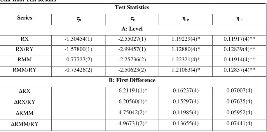
We first perform unit root tests in levels and first differences in order to determine univariate properties of the series used in this study. The results are presented in Table 1. It is evident from the table that the calculated ADF statistics are less then their critical values in all cases, suggesting that the variables are not level stationary. Table 1 also shows that the ADF statistics for the four variables imply first-difference stationary. The KPSS test, as indicated by the and statistics, rejects the I(0) null at the 95% and 90% respectively.

Table 1

Unit Root Test Results

Test Statistics

Series ττττµµµµ ττττττττ

A: Level

RX -1.30454(1) -2.55027(1) 1.19229(4)* 0.11917(4)**

RX/RY -1.57800(1) -2.99457(1) 1.12880(4)* 0.12839(4)**

RMM -0.77727(2) -2.25736(2) 1.22321(4)* 0.11914(4)**

RMM/RY -0.73426(2) -2.50623(2) 1.21063(4)* 0.12837(4)**

B: First Difference

∆RX -6.21191(1)* 0.16237(4) 0.07007(4)

∆RX/RY -6.20560(1)* 0.15297(4) 0.07635(4)

∆RMM -4.75042(2)* 0.11985(4) 0.05952(4)

∆RMM/RY -4.96731(2)* 0.13655(4) 0.07441(4)

Having established that all variables are integrated of the same order, we proceed with the Johansen multivariate cointegration tests, which allow us to test for long-run current account balance sustainability.

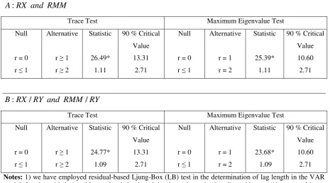
Before undertaking cointegration tests, let us first specify the relevant order of lags(p) of the vector autoregression (VAR) model. Lag order was determined using the residual-based Ljung-Box (LB) test. Lag in VAR model is 2 for the two models. The results obtained from the JJ method are presented in Table 2 below.

Table 2

Johansen-Juselius Maximum Likelihood Cointegration Tests

RMM and RX A:

Trace Test Maximum Eigenvalue Test

Null

r = 0

r 1

Alternative

r 1

r 2

Statistic

26.49*

1.11

90 % Critical

Value

13.31

2.71

Null

r = 0

r 1

Alternative

r = 1

r = 2

Statistic

25.39*

1.11

90 % Critical

Value 10.60 2.71 RY RMM and RY RX

B: / /

Trace Test Maximum Eigenvalue Test

Null

r = 0

r 1

Alternative

r 1

r 2

Statistic

24.77*

1.09

90 % Critical

Value

13.31

2.71

Null

r = 0

r 1

Alternative

r = 1

r = 2

Statistic

23.68*

1.09

90 % Critical

Value

10.60

2.71

Notes: 1) we have employed residual-based Ljung-Box (LB) test in the determination of lag length in the VAR model. Starting with k=1 and increasing k, lag length has been determined until reaching an unimportant Ljung-Box Q autocorrelation statistics belong to εt.

2) Asterisks (*) denotes statistical significance at 10%. r stands for the number of cointegrating vectors.

Turning to the maximum eigenvalue test, the null hypothesis of no cointegration (r = 0) is rejected at a 10 per cent level of significance in favour of the specific alternative, that there is one cointegrating vector, r = 1. However, the test fails to reject the null hypothesis of

r 1. This confirms the conclusion that there is only one cointegrating relationship amongst the two variables.

Thus, both the trace and the maximum eigenvalue test statistics reject the null hypothesis of r = 0 at the 10 per cent level of significance, and suggest that there is unique cointegrating vector. Therefore, our quarterly data from 1987 to 2002 appear to support the proposition that in Turkey there exist a stable long-run relationship of export and import plus net transfer payments and net interest payments.

Table 3

Estimates of Long-Run Cointegrating Vectors

RX RMM RX/RY RMM/RY

1.00 0.955 1.00 0.961

Estimates of long run cointegrating vectors are given in Table 3. For Turkey the estimated cointegrating vector is (1, 0.955) for real variables and (1,0.961) for real variables as a percentage of real GDP. For a sustainable relation, β should be equal to 1. The estimated cointegration factor, β, is significantly equal to 1. The empirical finding suggests that the current account of Turkey is sustainable in the long run.

Conclusion

REFERENCES

Ahmed, S., Rogers, J. H., (1995), “Government Budget Deficits and Trade Deficits. Are Present Value Constraints Satisfied in Long term Data.” Journal of Monetary Economics, 36(2), pp. 351-374.

Apergis, N., Katrakilidis, K.P., Tabakis, N.M., (2000), “ Current Account Deficit Sustainability: The Case of Greece.” Applied Economics Letters, 7, pp.599-603.

Dickey, D., Fuller, W. (1981), “The Likelihood Ratio Statistics for Autoregressive Time Series with a Unit Root.” Econometrica, 49, pp.1057-1072.

Fountas, S., Wu, J-L. (1999), “Are The U.S. Current Account Deficits Really Sustainable?”, International Economic Journal, 13(3), Autumn, pp.51-58.

Hakkio, C.S., Rush, M. (1991), “Is the Budget Deficit “Too Large?” Economic Inquiry, 39(July), pp.429-445.

Hamilton, J. D., Flavin, M.A. (1986), “On the Limitations of Government Borrowing: A Framework for Empirical Testing.” American Economic Review, 76(4), pp.808-819.

Husted S. (1992), “The Emerging U.S. Current Account Deficit in the 1980s: A Cointegration Analysis,” The Review Of Economics&Statics, February, pp. 159-166.

Johansen, S., Juselius, K., (1990), “Maximum Likelihood Estimated and Inference on Cointegration with Application to the Demand for Money.” Oxford Bulletin of Economics and Statistics, 52, pp.169-210.

Kwiatkowski, D., Philips, P.C.B., Schmidt, P., Shin, Y., (1992), “ Testing the Null Hypothesis of Stationary Against the Alternative of a Unit Root. How Sure Are We that Economic Time Series Have a Unit Root?” Journal of Econometrics, 54, pp.159-178.

MacKinnon, J. G., (1991), “Critical Value for Cointegration Tests.” in Engle, R.F., Granger, C.W.J., eds., Long-Run Economic Relationships: Reading in Cointegration. Oxford: Oxford University Press, pp.267-276.

Said, E. S., Dickey, D. A., (1994), “Testing for Unit Roots in Autoregressive-Moving Average Models of Unknown Order.” Biometrika, 71, pp.599-607.

Sawada, Y. (1994), “Are the Heavily Indebted Countries Solvent: Tests of Intertemporal Borrowing Constraints.” Journal of Development Economics, 45, pp.325-337.

Tanner, E., Liu, P., (1994), “Is the Budget Deficit ‘Too Large’: Some Further Evidence.”

Economic Inquiry, 32, pp. 511-518.

Trehan, B., Walsh, C. (1991), “Testing Intertemporal Budget Constraints: Theory and Applications to U.S. Federal Budget and Current Account Deficits.” Journal of Money, Credit, and Banking, 23 (2), pp. 206-223.