Size and Shape of Sample Units in Native Forests and Plantations

http://dx.doi.org/10.4236/ojf.2014.44043

How to cite this paper: Péllico Netto, S., Tello, J. C. R., & Wandresen R. R. (2014). Size and Shape of Sample Units in Native Forests and Plantations. Open Journal of Forestry, 4, 379-389. http://dx.doi.org/10.4236/ojf.2014.44043

Size and Shape of Sample Units in Native

Forests and Plantations

Sylvio Péllico Netto1*, Julio Cesar Rodriguez Tello2, Rafael Romualdo Wandresen3

1_{Department of Forest Science, University Federal of Paraná, Curitiba, Brazil} 2_{Department of Forest Science, University Federal of Amazonas, Manaus, Brazil}

3_{Department of Professional and Technological Education, University Federal of Paraná, Curitiba, Brazil} Email: *_{[email protected], [email protected], [email protected]}

Received 12 May 2014; revised 16 June 2014; accepted 5 July 2014

Copyright © 2014 by authors and Scientific Research Publishing Inc.

This work is licensed under the Creative Commons Attribution International License (CC BY). http://creativecommons.org/licenses/by/4.0/

Abstract

The size and form of sampling units-SU have always been variables considered in planning and structuring forest inventories, being performed in forests or in plantations. The experimental work outlined to deal with the problem was conducted in an area of araucaria forest, in Sao Joao de Triunfo, PR, Brazil. The forms of sampling units circle, square and rectangular were evaluated, whose areas ranged from 200 m2 _{to 1000 m}2_{. Time was recorded using a stopwatch and computed} separately for locomotion and measurement. The power model was used to adjust the relations of the times of locomotion and measurement, as well as a hyperbolic one for the coefficient of varia- tion, all taking as function of the SUs sizes. To achieve the analytical solution for the optimum size of the SU, it was necessary simulating the behavior of the three functions until the size of 10,000 m2_{. By taking the derivative of the combined function it was found the maximum point, which al-} lowed optimizing the size of the SU in 600 m2 _{for the structured experimental conditions. This} re-sult proved the formulated hypothesis, performing even a critical analysis of the inclusion of other relevant variables, such as size of the area to be inventoried, number of SUs performed in one day of work, average distance between the SUs, average speeds for locomotion between SUs and for taking all respective measurements.

Keywords

Optimization of the Size of Plots, Sampling of Fixed Area, Efficiency per Day of Work, Mixed Tropical Forest

1. Introduction

agement, being performed in plantations or in native forests. The information is usually obtained by sampling and this is taken in a sample space previously defined.

The sampling unit-SU, as it is specified a priori in its shape and size, characterizes a selection with probability proportional to the area and frequency of individuals who comprise it, and is called a method of Fixed Area.

It will be considered three relevant aspects that directly affect the size and shape of SUs: 1) The degree of va- riability of the experimental variable used to express the SU, usually the volume; 2) The costs or time spent to obtain the information in the SUs and 3). The degree of effectiveness to accomplish the work of data collection in minimal time.

It is known, of several published works in the field of forest inventory, that the shape and size of SUs has been decided much more by convenience and the operability of their location and demarcation in the field, than by analytical criterion (Péllico Netto & Brena, 1997; Silva, Xavier, Leite, & Pires, 2003). Whilst it is extremely valid worrying about the more appropriate conditions to sample forests or plantations, it will be equally relevant worrying about optimizing the time and the cost of the measurements as well as when conducting other activities in the sampling procedures.

Even the researchers dedicated to this theme, attempted to establish a close relationship between cost and time spent on activities of sampling to reach sizes and most appropriate ways of SUs, ceased to evaluate the influ-ences of biological variables and observe physical reality in each forest, such as size of the population used as a Production Unit (PU), logistic conditions in inaccessible areas and planning the activities to be carried out by the team of measurement, especially when their permanence in the field work is of limited durations. Although these latter variables are difficult to assess, they influence the final decision of this optimization process.

Pearce (1953), referring specifically to this problem, says there is a contradictory situation to reach an opti- mum size of the SUs, because the smaller units provide economy of time and larger ones provide economy of labor.

In fact, rectangular units have mostly been used in sampling the native forests. In addition to the better control of marginal trees, the detection of species diversity becomes a relevant aspect to this decision (Péllico Netto & Brena, 1997).

In forest inventories conducted in Europe, especially in Scandinavia, there is a strong preference for using small circular plots, whose decision fits into the context of Pearce (1953), i.e., given the small number of forest species occurring in the northern hemisphere and practicality in sampling with circular plots, whose radius do not exceed 3.5 meters, because, in these circumstances, you can easily use an aluminum rod to control border- line trees. In this sense, experiments carried out in Germany confirm that the circular plots up to size of 0.1 ha are more efficient to inventory native forests; when the plots, for some reason should be of larger sizes, it has been recommended the use of rectangular or square plots (Richter & Grossmann, 1951).

Messavage and Grosenbaugh (1956), working in field experiments in the north of Arkansas, in the United States, have used systematic sampling with plots arranged in rectangular structures (1:4), quadrangular (1:1) and random sampling with 16 plots of 1.6 acres in a population of 25.6 acres and held, in addition to the evaluation of accuracy of sampling, the evaluation of time spent for the measurements and for walking between the plots, aiming to compare finally the costs of these activities in the two structures of sampling.

To analyze the results of this work, the authors stated: 1) the efficiency of the sampling is the result of the joint evaluation of the cost and accuracy of the different sampling procedures used, i.e. it is a function of the re- ciprocal of the product of the square of the sampling error, given in percentage, by the cost. This is considered an optimal when the result is maximum; 2) citing Cochran (1963), they concluded that the systematic structure (1:1) resulted, for the same cost obtained, that the random sampling has an accuracy of the order of (1∕2)−0.5_{, and}

regarding the cost, for the same accuracy between both, the random sampling would cost twice as much as what it would be spend if used the systematic sampling; 3) confirmation of decrease of the coefficient of variation and sampling errors estimates with the increase of plot sizes; 4) efficiency was diverse, sometimes occurred to units of smaller sizes, sometimes to larger ones, which permitted the conclusion that is relevant introducing other va- riables sensitive to population variations, to make possible the obtainment of the optimum plot size for each for- est reality.

( )

1 2 x

E= T CV _− (1)

The circle shows, under the conditions mentioned above, minimization of occurrences of borderline trees, given this, among other geometric shapes of the same size, the one which has the smaller perimeter (Prodan, 1965), constituting this a first analytical contribution, for such circumstance, to decide the shape of the SU.

Smith (1938) was the precursor for the various scientific studies about size and shape of SUs, demonstrating that there is a negative exponential relationship between the plot size and the mean squared error obtained for the variable used to express it. This relationship, also known as an indicator of “Maximum Curvature”, does not reach a critical point to the choice of the plot size. Usually it is expressed using the coefficient of variation as a function of the size of the SU.

Many researchers have tried to explain scientifically this exponential reduction, because if the coefficient of variation is the ratio between the standard deviation and the mean of the estimated X variable, and being both obtained in the same unit of measurement, it was expected that by doubling the size of the SU, both statistics should double their sizes and, consequently, the coefficient of variation should be constant.

It was only with the work presented by Loetsch, Zöhrer and Haller (1973) that such reduction theoretically was explained. This relationship is expressed by σ = σ2y 2 2x

(

1+ ρ

)

, in which

2 y

σ is the variance of SU of folded size of that used to obtain σ2x, and ρ the correlation coefficient between measured values taken in adjacent SUs

of the same size. By transforming such relation in terms of coefficients of variation and doubling the size of SUs that 2 2

(

)

(

)

2

1 2

1

2 x 4

CV = σ +ρ X − , or simplifying the equality it results in

(

)

( )

2 2

2

1 2

1

2 x 4

CV = σ +ρ X − , or still considering any increase in size of SUs

( )

W the equality finally results in

(

)

1 2

2 1 1

CV =CV _ +ρ W_ .

Note that CV2 will only be twice the CV1 when ρ =1, occurring for units of expressive sizes. Queiroz

(2011)working in the Tapajos National Forest, PA, Brazil, has selected the species Manilkara huberi and stu- died SUs of growing sizes between 400 m2 up to 10,000 m2, having obtained the function adjusted for the coef- ficient of variation CV2 =1134.9198A−0.7044998, as was firstly suggested by Lessman and Atkins (1963), in which A is entered directly in m2. During this experiment the assessment of correlation coefficient reached the value of 0.720 for the size of 10,000 m2, indicating that ρ =1 only will be reached for sizes larger than 1 hec- tare.

Péllico Netto (1979), considering the suggestions made by Messavage and Grosenbaugh (1956), has proposed to increase the number of variables to achieve an optimum size for the SU, including: 1) Size of the area to be inventoried—Af; 2) Time for locomotion or displacement between SUs—T1; 3) Measuring time of the SUs—T2

and 4) The number of hours per day worked by the measurement team—T3. This proposal is based on the con-

cept of Efficiency per Day of Work-EDT, which is based on the equation used in physics to obtain speed as a function of space and time and is strictly related to the size of the SU, expressed by:

(

)

1

(

)

(

)

2

1 1 1

1 2

EDT=_ A n_f − n_d+1_v− + An_d v−

  (2)

where: n= sample size; n_d = sample size per day of work; A= area of the SU; v₁= speed of locomotion between SUs and v₂ = speed of taking measurements in the SUs.

Note that the concept of EDT is equivalent to the time T3, i.e., the time spent in locomotion and in measure-

ments on a day of work. If this working time, optimistically, is always close to 8 hours actually worked in a day of work, then aforciori the inventory as a whole will be optimized.

Zaide (1980) also considered time as important variable for plot size optimization and stated that the optimum achievement is reached when the time is minimum for the execution of activities of installation and measure- ment of the SUs with accuracy established for the variable considered in the sampling (usually the volume). Therefore, any experiment performed to achieve optimization of the SUs depends on the total time in function of the size of the SUs and consider such variations in a relationship that will allow minimizing the total time of measurement.

Therefore the total time for the day of work can be expressed by:

(

)

3 1 2 1 2

1 1 1

h h h

n n n

di di di

i i i

T n T n T n T T

= = =

where: T3= total time in a day of work; T1= average time of locomotion and T2 = average time of

mea-surement.

As proposed by Péllico Netto (1979), it can be observed that the time of locomotion T1 is equated by:

(

)

1

(

)

2

1 1

1 f d 1 1

T =_ A n− n + _v−

  (4)

Or:

(

)

(

)

2

2 1 2

1 f d 1 1

T =_ A n− n + _v− (5)

The same way, the time of measurement may be taken as:

(

)

1

2 d 2

T = An v− (6)

Given the theoretical content, the objective of this work was to integrate such knowledge experimentally to test the following hypothesis: It is possible to derive an analytical solution for a more appropriate size of the sample unit-SU and effective to be used in all types of forest inventories.

2. Materials and Methods

The data used to illustrate the present process of obtaining the size of SUs were collected in a native forest of Araucaria angustifolia, located in Sao Joao do Triunfo, PR, at an altitude of 780 m (25˚34'18" Latitude and 50˚05'56" Longitude W), belonging to the Federal University of Parana, with 32 ha (Tello, 1980) and will be mentioned later as araucaria experiment—AE.

The demarcation of the experimental area was performed considering the topography and edaphic conditions the most uniform possible, to allow comparisons between shapes, sizes and time spent for measurements of SUs, so that they could be performed with maximum similarity.

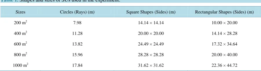
The experimental area was delimited in nine fields, each with one hectare, in which were laid down the varia- tions of sample structure more commonly used in forest inventories, i.e.: circle, square and rectangular SUs, with variations from 200 m2 up to 1000 m2, as is shown in Table 1.

After demarcations of the SUs, DBH, total and commercial heights of all trees were collected, being that for Araucária (DAP ≥ _{10 cm) and for the other species (DBH} ≥ _{20 cm).}

The equations used for obtaining the volume per species are presented in Table 2.

The sample which was applied to each size of SUs came from a pilot inventory to have the preliminary esti- mators of mean and variance of various shapes and sizes of SUs, to what it has been established an error limit of 10% of the average volume with 95% probability. The results for a sampling area of 9 ha are presented in Table 3.

The time spent for each one of the activities carried out in the SUs were obtained using a stopwatch and computed individually, as suggested by Stöhr (1978), to prevent the operations of subtraction performed to ob- tain the liquid times by activities, when using continuous timing. The result of this operation is shown in Table 4.

[image:4.595.86.537.600.723.2]

Tello (1980) using such obtained estimators and having them applied in Equation (1) proposed by Freese (1962) concluded that the maximum efficiency in all forms occurred with the size of 1000 m2 with a small ad- vantage for the circular shape, which minimized the total time for this size. This conclusion clearly shows that

Table 1. Shapes and sizes of SUs used in the experiment.

Sizes Circles (Rays) (m) Square Shapes (Sides) (m) Rectangular Shapes (Sides) (m)

200 m2 7.98 14.14 × 14.14 10.00 × 20.00

400 m2 _{11.28 20.00 × 20.00 14.14 × 28.28}

600 m2 _{13.82 24.49 × 24.49 17.32 × 34.64}

800 m2 _{15.96 28.28 × 28.28 20.00 × 40.00}

[image:5.595.88.538.191.302.2]

Table 2. Equations adjusted for calculations of tree volumes in the SUs.

Species Equations

Araucaria (Total Volume) v=0.02394804+0.5330851d h2

Araucaria (Commercial Volume) _{v= −0.0515975−0.623586d}2_{+0.7749955d h}2 _{−0.009742885dh}2_{+0.001808991h}2 Other species (Commercial Volume) lnv= −0.16984+2.15797 lnd+0.73378 lnh

Table 3. Sample sizes demanded for sampling and average distance (D) between the SUs.

Size (m2₎ Circle Shape Square Shape Rectangular Shape

n D (m) n D (m) n D (m)

200 135 25.82 120 27.38 166 23.28

400 69 36.12 62 38.10 62 38.10

600 43 45.75 46 44.23 42 46.29

800 29 55.71 32 53.03 30 54.77

1000 24 61.24 23 62.55 21 65.47

Note: n = sample size, D = average distance between SUs.

Table 4. Average speeds for locomotion, measurements and total in different sampling schemes.

Form Size (m2) Locomotion _(Minutes) Measurement _{(Minutes) (Minutes)} Total

Average Speeds

nd v1 (m∙h−1) v2 (m2∙h−1)

Circle

200 08.65 09.92 18.57 179.10 1209.67 25

400 10.01 20.54 30.55 216.50 1168.45 15

600 11.13 33.54 44.67 246.63 1073.35 10

800 13.70 45.55 59.25 243.99 1053.79 08

1000 14.20 53.45 67.65 258.76 1122.54 07

Average 1125.56

Square

200 08.99 16.50 25.49 182.74 727.27 18

400 10.85 28.21 39.06 210.69 850.76 12

600 11.03 43.95 54.98 240.60 819.11 08

800 13.10 58.19 71.29 242.88 824.88 06

1000 14.30 67.55 81.85 262.45 888.23 05

Average 822.05

Rectangular

200 08.32 15.50 23.82 167.88 774.19 20

400 10.85 27.61 38.46 210.69 869.25 12

600 11.16 42.95 54.11 248.87 838.18 08

800 13.25 53.59 66.84 248.02 895.69 07

1000 14.45 68.85 83.30 271.85 871.46 05

Average 849.75

[image:5.595.90.536.343.660.2]

rimental conditions.

The simulation was structured using the mathematical models: power for the times and a hyperbole for the coefficient of variation, as is shown in Table 5.

The estimate of the total time was calculated by the sum of the estimators of the times of locomotion and measurement, as presented in Equation (7):

1 2

ˆ ˆ ˆ

T

T = +T T (7)

where: TˆT Estimator of total time (minutes).

The estimate of relative efficiency was calculated using the Equation (1). If TˆT and CV is replaced by

their respective mathematical models in (1) it becomes a function of the area of the SU.

(

1 3

)

(

1

)

2

0 2 4 5

ˆ b b

E= b A +b A b +b A− − (8)

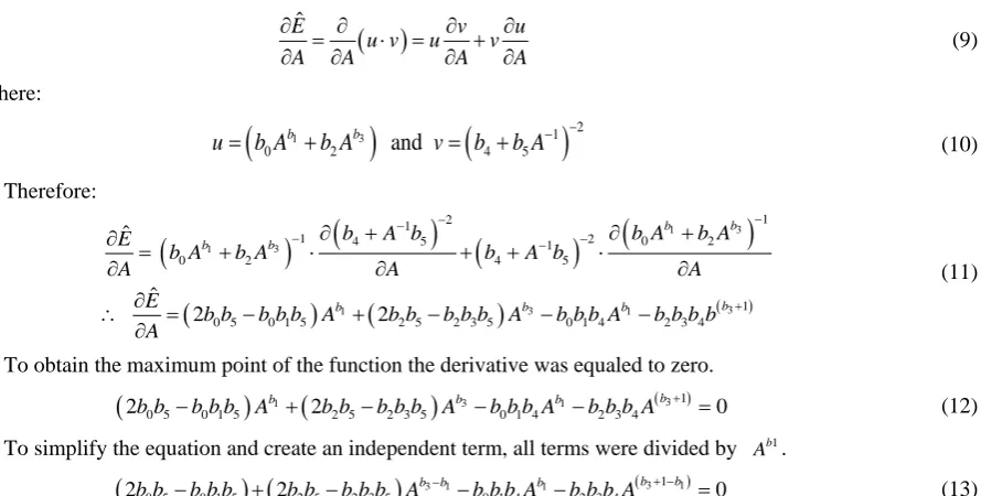
The derivative of _Eˆ _{was taken in relation to A and the result was equated to zero to obtain the highest}

ef-ficiency for the size of the SU. Considering additionally the derivative of a product:

( )

ˆ

E v u

u v u v

A A A A

∂ ∂ ∂ ∂

= ⋅ = +

∂ ∂ ∂ ∂ (9)

where:

(

1 3

)

(

1

)

2

0 2 and 4 5

b b

b A b A v b b A

u= + = + − − (10)

Therefore:

(

) (

) (

)

(

)

(

)

(

)

( ) 3 1 3 1 3 3 1 1 1 2 1

1 4 5 ₁ 2 0 2

2 4 5

1 0 5 0 1 5 2 5 2 3 5 0 1 4 2 3 4 0 ˆ ˆ 2 2 b b b b b b b b b A E b A

A A A

E

b b A b b

b A A

b b

b A A b b

b b b b b b A bb b A bb bb

A − − − − ₋ − + ∂ + ∂ + ∂ = + + + ∂ ∂ ∂ ∂ ∴ = − + − − ⋅ − ∂ ⋅ (11)

To obtain the maximum point of the function the derivative was equaled to zero.

(

)

1

(

)

3 1 (3 1)

0 5 0 1 5 2 5 2 3 5 0 1 4 2 3 4

2bb −bb b Ab + 2bb −bb b Ab −bb bAb −bb b Ab+ =0 (12) To simplify the equation and create an independent term, all terms were divided by b1

A .

(

) (

)

3 1 1 (3 1 1)

0 5 0 1 5 2 5 2 3 5 0 1 4 2 3 4

2bb −bb b + 2bb −bb b Ab−b −bb b Ab −bb b Ab+ −b =0 (13) The value of the area

( )

A in the equation, because the algebraic complexity to isolate it, was calculated us-ing the function Solve of the mathematical software Matlab.

3. Results

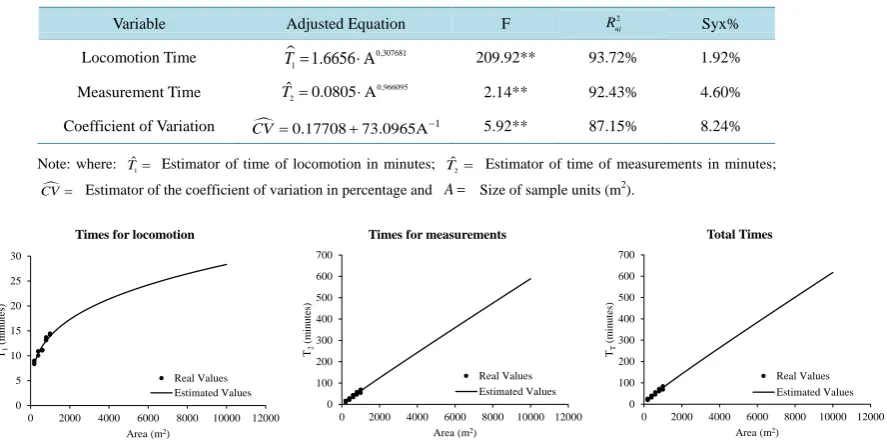
The equations adjusted and the statistics of the regression for the times of locomotion, measurements and coeffi-cient of variation, obtained with the adjustment of the models shown in Table 5, are presented in Table 6. The estimate of the total time was calculated by the sum of these estimators using Equation (7), and is presented in

[image:6.595.95.540.262.487.2]

Figure 1.

Table 5. Mathematical models used.

Variable Model used

Time of locomotion 1

1 0

ˆ b

T =b A

Time of taking measurement 3 2 2

ˆ b

T =b A

Coefficient of Variation  1 4 5

CV=b +b A−

Note: where: Tˆ1= estimated time of locomotion (minutes); Tˆ2= Estimated time of measurements (minutes); A=

Size of sampling units (m2_{); }

[image:7.595.94.538.98.322.2]

Table 6. Adjusted Equations and statistics for T1, T2 and CV.

Variable Adjusted Equation F 2

aj

R Syx%

Locomotion Time  0,307 1

681 1.6656 A

T= ⋅ 209.92** 93.72% 1.92%

Measurement Time 0,966 95 2

0

0.0805 A ˆ

T = ⋅ 2.14** 92.43% 4.60%

Coefficient of Variation _CV_{=0.17708+73.0965A}−1 _{5.92** 87.15% 8.24%}

Note: where: Tˆ1= Estimator of time of locomotion in minutes; Tˆ2= Estimator of time of measurements in minutes;



[image:7.595.94.539.208.317.2]

CV= Estimator of the coefficient of variation in percentage and A= Size of sample units (m2_).

Figure 1. Estimate of the times for locomotion, measurements and total.

Figure 1 presents the estimate of times for locomotion

( )

T1 , for measurements

( )

T2 and total

( )

TˆT in re-

lation to the size of sample units. The dots represent the values observed for the sizes of plots of 200, 400, 600, 800 and 1000 m2 for shapes: circle, square and rectangular. The curve represents the values estimated for the sizes up to 10,000 m2.

Figure 2 shows the correlation coefficient in relation to the size of the SUs. The dots represent the values measured in the SUs of the sizes 200, 400, 600, 800 and 1000 m2 for shapes: circle, square and rectangular. The prognosis was made for sizes up to 10,000 m2.

The relative efficiency

( )

Eˆ , using the Equation (1), was obtained by means of the estimates of the total time

( )

ˆ

T

T and the estimate of the coefficient of variation

( )

CV .

Figure 3 shows the graph obtained for the relative efficiency in relation to the size of the SUs. The dots represent the actual values measured for the sizes of the SUs of 200, 400, 600, 800 and 1000 m2, for shapes: cir- cle, square and rectangular. The curve represents the values estimated for the sizes up to 2200 m2.

The graph in Figure 3 shows that, for the analyzed data, the plot size of better efficiency (around 0.2203) is approximately 600 m2.

Substituting in Equation (13) the values of the coefficients obtained by the adjustment of the models listed in

Table 6, we obtained the following result:

0.6584 1.6584

206.0392 6.0837+ A −0.0138A −0.0907A=0 (14)

It was used to solve the function Matlab software, as is shown in Figure 4. Thus, for the analyzed data, the plot size with better efficiency is of 604.11 m2.

The form of SUs was analyzed considering the minimum total time spent to locate and measure them. As they are presented in Table 4, the average total time to perform the sampling with the SU of 600 m2 was of 44.67 minutes, 54.98 minutes and 54.11 minutes for the SUs circle, square and rectangular shapes, respectively, meaning that the circle is clearly the best shape to be used in the forest conditions observed in the experiment. In Europe and also in the United States the majority of productive forests is conducted using the natural regenera- tion as a silvicultural methods, hence its appearance is approaching the structure of native forest, then the circle is widely distributed and used in forest inventories in both regions (Péllico Netto & Brena, 1997), but it is worth mentioning that European authors limit the size of the units to 0.1 ha, because they can measure more units of smaller size, better detect the variability within the sampled area and reduce the edge effect in this form of SU

(Strand, 1957).

For sizes larger than 0.1 ha is advisable to use the rectangular units, because its efficiency increases due to 0 5 10 15 20 25 30

0 2000 4000 6000 8000 10000 12000

T1

(m

inut

es

)

Area (m2)

Times for locomotion

Real Values Estimated Values 0 100 200 300 400 500 600 700

0 2000 4000 6000 8000 10000 12000

T2

(m

inut

es

)

Area (m2₎

Times for measurements

Real Values Estimated Values 0 100 200 300 400 500 600 700

0 2000 4000 6000 8000 10000 12000

TT

(m

inut

es

)

Area (m2)

Total Times

[image:8.595.124.480.91.522.2]

Figure 2. Coefficient of variation.

Figure 3. Relative efficiency.

Figure 4. Analytical solution for the optimum size of SU obtained by Matlab software.

better control of edge effects, as well as favoring the detection of species diversity in native forests. In the case of forest plantations, due to the regularity of the lines of plantations and the spacing between trees, the research- ers prefer to use the rectangular shape of SU, for ease of installation and demarcation of the SU, mainly when applying successive sampling in continuous forest inventories (Cesario, Engel, Finger, & Schneider, 1994; Simplício, Muniz, Aquino, & Soares, 1996; Strand, 1957).

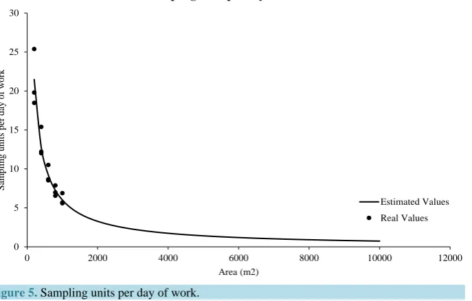
The maximum amount of sample units per day of work

( )

nd was obtained by means of the estimates of the

average total time to measure a SU

( )

TˆT and the estimate of the average time of locomotion between two SUs



( )

T1 , as considered in (15).

(

)

1

1

ˆ

480 ˆ_T

nd= −T ⋅T− (15)

Figure 5 shows the maximum amount of sample units capable of being performed in one day of work (8 hours) for each size of SU. The dots represent the values measured for the plot sizes of 200, 400, 600, 800 and 1000 m2, for shapes: circle, square and rectangular. The curve represents the values estimated for the sizes up to 10,000 m2.

The graph in Figure 5 and by means of the obtained data, it is noted that the largest possible sample unit to be

0% 10% 20% 30% 40% 50% 60%

0 2000 4000 6000 8000 10000 12000

C

o

ef

fic

ie

n

t

o

f v

ar

ia

tio

n

Area (m2₎

Coefficient of variation

Estimated Values

Real Values

0,12 0,14 0,16 0,18 0,20 0,22 0,24 0,26

0 500 1000 1500 2000 2500

R

el

at

iv

e E

ff

ici

en

cy

Area (m2₎

Relative Efficiency

Estimated Values

[image:9.595.132.476.96.315.2]

Figure 5. Sampling units per day of work.

measured in 8 hours (one day of work), for this data set, is 7000 m2.

The simulations using the integration of the assessed variables permitted the optimization, by means of an analytical process to obtain the most appropriate plot size for the sampling conditions used in the forest popu- lation, in this case 600 m2, which proves the formulated hypothesis. Such procedure was possible, however, due to some relevant aspects detected in structuring this process: 1) it was not possible to derive Equation (8) using the power function for expressing the relationship of CV with the plot sizes, although it has been used in many scientific works since its proposition by Lessman and Atkins (1963). It was due to the proposed use of a hyper- bolic function by the authors which became possible the functionality of the analytical process until obtaining the optimum plot size; 2) Although this analytic solution has already been formalized by Zaide (1980), using the power functions for the three variables of the process (times of locomotion and measurements, and coefficient of variation), he succeeded because he determined the power values of such functions. When we obtained them by adjusting a linear regression model, the derivative process did not work.

Applying the experimental results in Equation (2) it was possible to get the value of EDT=13.29 hours, a result not doable in a day of work. This shows that only the process of statistical optimization, which involves the inclusion of times for locomotion, measurements and reduction of the coefficient of variation as a function of plot size, cannot optimize also the performance of the sampling in a day of work, which should not exceed 8 hours.

Cesaro et al. (1994) compared fixed area plots with the Bitterlich and Prodan SUs in Rio Grande do Sul, hav- ing assessed carefully the times of location, installation and measurements of dbh and height of the trees in an area of 4.6 ha for the three sampling methods. They used a fixed area plot of 600 m2, which allowed compari- sons with the results obtained in this work, in spite of their experiment have been conducted in stands of Pinus sp., with 28 years of age, which will be referenced later as pine experiment—PE.

In the PE, after having performed the calculation of the estimators needed for comparative purposes, the av- erage distance between the units of fixed area sampled resulted in D=71.49 m, the average time of locomotion between the SUs was 5.35 minutes and, consequently, the average speed of locomotion between them was

1 1 801.75 m hour

v = ⋅ − . The average time spent for the measurements in the SUs was 19.94 minutes and, conse- quently, the average speed of the measurements of them was v2 1,805.42 m hora2 1

−

= ⋅ . Effectuating the calcula-tion with the formulacalcula-tions presented in this work, it was found that the total time spent to sample 9 SUs of 600 m2 was 227.55 minutes and the average time to measure a unit was 25.29 minutes. Considering these results, you may ask: What is the number of SUs that could be performed in a day of 8 hours of work

( )

nd , aiming to

optimize the data collection? This result can be obtained by applying the Equation (15), which results in 18

d

n = plots. Although the speeds for locomotion and for measurements obtained by them have been larger than those observed in AE Table 4, in which the average distance for rectangular units of 600 m2 was only

0 5 10 15 20 25 30

0 2000 4000 6000 8000 10000 12000

S

am

pl

in

g

u

n

it

s pe

r

da

y

of

w

or

k

Area (m2)

Sampling units per day of work

Estimated Values

46.29 m

D= (Table 3), it becomes understandable why the number of units appropriate to be performed in 8 hours was only 8 SUs (Table 4).

In several forest inventories of companies carried out in pine plantations have been reported that such effi- ciency is possible, however it is worth noting that the conditions of access and the level of experience of the field teams should be very good. In most adverse conditions of access the average velocities, both for locomo- tion or for measurement, tend to be smaller. Still, as discussed in the AE, such number of SUs per day of work was obtained without the incorporation of the variable coefficient of variation.

This type of experiment can be repeated both in natural forest, as well as in plantations to define the appropri- ate plot size to be used in the forest inventory, however, from a practical point of view, it can be assumed, at the light of the result obtained in the AE, the constraints that will allow approaching to the optimum plot size, mainly in the case of plantations.

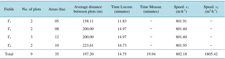
Faced with the premise that such evaluation can be performed with the same effectiveness by the sampling team in one day of work (EDT), it is not relevant anymore to focus on planning of the forest inventory as a whole, and what is important to be known is summarized in Table 7.

The area of the company to be measured is 35 ha, with four compartments, which has two or three plots in each one of them. It will be assumed that the company has performed a timing to see about the times spent for locomotion between the plots and also to perform the measurements of all dbh and heights of a percentage of trees. With these data at his disposal it is possible to calculate the speeds for locomotion and measurement and can also clearly specify in its planning that the team must work 8 hours per day performing the sampling activi- ties.

Using the result obtained previously nd =18 and isolating the size of the plots (A) into (2) we have:

(

)

1

(

)

2

1 1

1 1

8 f d d 1 ( d)

A=_ v − A n− n + _ v n − _

 

  (16)

Replacing it in the data of Table 7 in (16) we have:

( )

(

1

)

12

(

)

( )

1

2

8 802.18 350, 000 18 18 1 802.18 18 1805.42

471.14 m

A

A

− −

  

=_ × − × × + _{ } × _ ×

 

 

∴ =

(17)

As noted, when it was expanded the number of variables in the decision-making process to decide what is the optimum size of SU, the measurement of 18 SUs per day allows you to measure units of only 471.14 m2 which can be rounded up to 470 m2. However, if the company believes that the unit of 600 m2 should be maintained as the best option, they may reduce the number of units to be measured in a day of work

( )

nd to optimize also the

efficiency of the field work. In many forest companies teams trained in forest inventories of pine or eucalyptus plantations can measure up to 18 plots per day. This is an exceptional situation, however 15 plots per day is a quantity considered very good. Recreating the calculations in (16) we have:

( )

(

)

1

(

)

[

]

2 1

1

8 802.18 350, 000 15 15 1 802.18 (15) 1805.42

A=_ × − × − × + _ × − _×

 

  (18)

2

596.18 m

[image:10.595.87.538.599.718.2]

A= , an approximate value of 600 m2, which was the optimum size obtained at AE and used in PE.

Table 7. Preliminary data collected by the company for definition of the optimum size of the SU.

Fields No. of plots Areas (ha) Average distance between plots (m)

Time Locom. (minutes)

Time Measur. (minutes)

Speed. v1

(m∙h-1

)

Speed. v2

(m2∙h-1)

T1 2 05 158.11 11.83 ̶ 801.91 ̶

T2 2 08 200.00 14.97 ̶ 801.60 ̶

T3 3 12 200.00 14.97 ̶ 801.60 ̶

T4 2 10 223.61 16.73 ̶ 801.95 ̶

4. Conclusion

The hyperbolic function proposed by the authors to express the coefficient of variation as a function of plot size became the possible functionality of the analytical process to obtain the optimum plot size;

The simulation using the integration of the assessed variables permitted to get the optimization, and the most appropriated plot size for the sampling conditions of that forest population was 600 m2;

The use of additional variables as size of the area to be inventoried −A_f, time for locomotion or displace- ment between SUs—T1, measuring time of the SUs—T2 and the number of hours per day worked by the mea-

surement team—T3 made it possible to reach the Efficiency per Day of Work-EDT, which was based on the

eq-uation used in physics to obtain speed as a function of space and time and was strictly related to the size of the SU and, consequently, it was possible to verify that only the process of statistical optimization could not assure also the performance of the sampling in a day of work, which should not exceed 8 hours;

Applying the combination of the two procedures: optimization process and EDT evaluation, it was possible to obtain the most appropriate number of plots of 600 m2 to be measured in one day of field work, which in the case were 15 plots.

References

Cesario, A., Engel, O., Finger, C., & Schneider, P. (1994). Comparação dos métodos de amostragem de área fixa, relascopia

e de seis árvores, quanto a eficiência, no inventário florestal de um povoamento de Pinnus sp. Ciência Florestal, 4, 97-

108.

Cochran, W. (1963). Sampling Techniques (2 ed.). New York: John Wiley and Sons Inc.

Freese, F. (1962). Elementary Forest Sampling. Washington: US Department of Agriculture.

Lessman, K., & Atkins, R. (1963). Optimum Plot Size and Relative Efficiency of Lattice Designs of Grain Sorghum Yield

Test. Crop Science, 3, 477-481. http://dx.doi.org/10.2135/cropsci1963.0011183X000300060006x

Loetsch, F., Zöhrer, F., & Haller, K. (1973). Forest Inventory (2 ed., Vol. II). Munich: BLV Verlagsgesellchaft.

Messavage, C., & Grosenbauch, L. (1956). Efficiency of Several Cruising Designs on Small Tracts in North Arkansas. Journal of Forestry, 54, 569-576.

Pearce, S. (1953). Field Experiments with Fruit Trees and Other Perennial Plants. Technical Communication No. 23, East

Malling:Commonwealth Agricultural Bureaux.

Péllico Netto, S. (1979). Die Forstinventuren in Brasilien: Neue Entwiecklungen und ihr Beitrag für eine geregelte Forst-

wirtschaft. Mitteilungen aus dem Arbeitskreis für Forstliche BIOMETRIE. Freiburg: Tese de Doutorado, Albert-Ludwigs- Universität zu Freiburg im Breisgau.

Péllico Netto, S., & Brena, D. A. (1997). Inventário Florestal. Curitiba: Federal University of Paraná Press.

Prodan, M. (1965). Holzmesslehre. Frankfurt: J.D. Sauerländer’s Verlag.

Queiroz, W., Péllico Netto, S., Valente, M., & Pinheiro, J. (2011). Análise Estrutural da Unidade Conglomerada Cruz de

Malta na Floresta Nacional do Tapajós, Estado do Pará, Brasil. Floresta, 41, 9-18.

Richter, A., & Grossmann, H. (1951). Untersuchungen über Prokreis Gröβe und Netz Punktdichte bei Holzvorratsinventuren.

Archiv für Forstwesen,Heft 11.

Silva, R., Xavier, A., Leite, H., & Pires, I. (2003). Determinação do tamanho ótimo da parcela experimental pelos métodos da máxima curvatura modificado, do coeficiente de correlação intraclasse e da análise visual em testes clonais de eucalipto. Revista Árvore, 27, 669-676. http://dx.doi.org/10.1590/S0100-67622003000500009

Simplício, E., Muniz, J., Aquino, L., & Soares, A. (1996). Determinação do tamanho de parcelas experimentais em povoa-

mentos de Eucalyptus grandis Hill ex-Maiden: I, parcelas retangulares. CERME, 2, 53-65.

Smith, H. (1938). An Empirical Law Describing Heterogeneity in the Yields of Agricultural Crops. Journal of Agricultural

Science, 28, 1-23. http://dx.doi.org/10.1017/S0021859600050516

Stöhr, G. W. (1978). Importância e aplicação do estudo do trabalho. Floresta, 9, 27-38.

Strand, L. (1957). The Effect of the Plot Size on the Accuracy of Forest Surveys. Meddelelser fra det Norske skogforsøks-

vesen, 48, 621-649.

Tello, J. (1980). Eficiência e Custos de Diferentes Formas e Tamanhos de Unidades de Amostra em uma Floresta Nativa de

Araucaria angustifolia (Bert.) O. Ktze no Sul do Brasil. Dissertação de Mestrado, Curitiba: Universidade Federal do Paraná.