Munich Personal RePEc Archive
Evaluating Neural Spatial Interaction
Modelling by Bootstrapping
Fischer, Manfred M. and Reismann, Martin
Vienna University of Economics and Business, Vienna University of
Economics and Business
2000
Online at
https://mpra.ub.uni-muenchen.de/77790/
Evaluating Neural Spatial Interaction
Modelling by Bootstrapping
Manfred M. Fischer
Martin Reismann
Department of Economic Geography & Geoinformatics,
Vienna University of Economics and Business Administration
Rossauer Lände 23, A-1090 Vienna, Austria
Paper presented at the 6th World Congress
of the Regional Science Association International,
Abstract
This paper exposes problems of the commonly used technique of splitting the available
data in neural spatial interaction modelling into training, validation, and test sets that
are held fixed and warns about drawing too strong conclusions from such static splits.
Using a bootstrapping procedure, we compare the uncertainty in the solution stemming
from the data splitting with model specific uncertainties such as parameter
initialization. Utilizing the Austrian interregional telecommunication traffic data and
the differential evolution method for solving the parameter estimation task for a fixed
topology of the network model [ i.e. J = 9] this paper illustrates that the variation due to
different resamplings is significantly larger than the variation due to different parameter
initializations. This result implies that it is important to not over-interpret a model,
estimated on one specific static split of the data.
Keywords: Neural spatial interaction modelling, model evaluation, bootstrapping,
1. Introduction
Spatial analysis in currently entering a period of rapid change leading to what is termed
intelligent spatial analysis, sometimes referred to as geocomputation. The driving
forces are a combination of huge amounts of digital spatial data from the GIS data
revolution, the availability of attractive softcomputing tools, the rapid growth in
computational power, and the new emphasis on exploratory data analysis and
modelling. Intelligent spatial analysis has the following properties. It exhibits
computational adaptivity, computational fault tolerance in dealing with incomplete,
inaccurate, distorted, missing, noisy and confusing data; speed approaching human-like
turnaround and error rates that approximate human performance. The use of the term
’intelligent’ is, thus, closer to that in computational intelligence than in artificial
intelligence. The distinction between artificial and computational intelligence is
important because our semantic descriptions of models and techniques, their properties,
and our expectations of their performance should be tempered by the kind of systems
we want, and the ones we can build.
Much of the recent interest in intelligent spatial analysis stems from the growing
realization of the limitations of conventional spatial analysis tools as vehicles for
exploring patterns in data-rich GI (geographic information) and RS (remote sensing)
environments and from the consequent hope that these limitations may be overcome by
judicious use of computational intelligence technologies such as evolutionary
computation and neural network modelling. Neural network models may be viewed as
non-linear extensions of conventional statistical models that are applicable to two major
domains: first, as universal approximators to areas such as spatial regression, spatial
interaction, spatial choice and space-time series analysis; and second, as pattern
recognizers and classifiers to intelligently allow the user to sift through the data, reduce
dimensionality, and find patterns of interest in data-rich environments.
Neural spatial interaction models are termed neural in the sense that they are based on
neural computational models, inspired by neuroscience. They are more closely related
to spatial interaction models of the gravity type, and under commonly met conditions
they can be understood as a special class of general feedforward neural network models
networks can provide approximations within an arbitrary precision (i.e. it has universal
approximation property), as proven by Hornik et al. (1989).
Learning from examples, the problem for which neural networks were designed for to
solve, is one of the most important research topics in computational intelligence. A
possible way to formalize learning from examples is to assume the existence of a
function representing the set of examples and, thus, enabling to generalize. This can be
called a function reconstruction from sparse data (or in mathematical terms, depending
on the required precision, approximation or interpolation problem, respectively). Within
this general framework, the main issues of interest are the representational power of a
given network model and the procedures for obtaining the optimal network parameters.
It is the objective of this article to evaluate the out-of-sample or forecast performance of
neural spatial interaction approximators in a real world application environment.
Training a neural spatial interaction model is not hard, but once we have a spatial
interaction approximator, how much can we trust the forecast for truly new data? A
standard procedure for evaluating the performance is to split the data into one training
set (used for parameter estimation, e.g., through gradient descent or the differential
evolution method), one validation set (used to determine the stopping point before
overfitting occurs and/or used to set additional parameters or hyperparameters, such as
the importance given to the amplification of the differential variation in the case of the
differential evolution method), and one test set. This procedure has been used for many
years in the connectionist community [see, e.g., Weigend et. al. (1990) in general and in
neural spatial interaction modelling in particular [see Fischer and Gopal (1994)]. Recent
experience has found this approach, along with conclusions drawn from it, to be very
sensitive to the specific splitting of the data [see, Fischer and Gopal (1994)]. Thus,
usual tests of forecast reliability appear over-optimistic in general.
This paper addresses the problem of evaluating a neural spatial interaction model with a
bootstrapping procedure. The approach we present combines the purity of splitting the
data into three disjoint sets - as suggested in Fischer and Gopal (1994) - with the power
of a resampling procedure. This allows us to get a better statistical picture of forecast
variability, including the ability to estimate the effect of the randomness of the splits of
compare the uncertainties in the solution stemming from the data splitting with neural
network specific uncertainties such as parameter initializations. To demonstrate the
procedure, we use the Austrian interregional telecommunication traffic data and the
differential evolution method, a randomized parallel multipoint search procedure, for
solving the parameter estimation task as suggested in Fischer et al. (1999).
The remainder of the paper is as follows. The next section provides a summarized
description of single hidden layer neural spatial interaction models followed by a brief
characteristic of the training procedure used for determining the model parameters.
Section 4 describes the experimental design and the bootstrapping procedure while
section 5 presents the empirical results of the study. The final section draws some
conclusions.
2. Neural Spatial Interaction Predictors
Suppose we are interested in approximating an N-dimensional spatial interaction
function, where ℜN →ℜ
:
) , where ℜN
as N-dimensional Euclidean real space is the
input space and ℜ as 1-dimensional Euclidean real space is the output space. This
function should estimate spatial interaction flows from regions of origin to regions of
destination. In practice, only bounded subsets of the space are considered.
The function ) is not explicitly known, but given by a finite set of samples S = {zk= (xk,
yk), k = 1,..., K} generated by a process that is governed by ), that is )(xk) = yk, k = 1,...,
K. The set S is the set of pairs of input and output vectors. The role of network
modelling is to provide a specific form of a continuous function which approximates
(or interpolates) set S. The advantages of neural network modelling have to do with the
virtues associated with such specific forms.
To approximate ), we consider the class of neural spatial interaction models Ω with one
hidden layer, N input units, J hidden units and one output unit. Ω consists of a
. x w w y J j n n jn j j ϕ = =
∑
∑
=0 =0
) , ( ) ,
(x w x w (1)
Vector x = (x1,..., xN) is the input vector augmented with a bias signal x0 which can be
thought as being generated by a ‘dummy unit’ whose output is clamped at 1. The wjn's
represent input to hidden connection weights and the wj's hidden to output weights
(including the bias). The symbol w is a convenient shorthand notation of the
d = (J (N + 1) + J + 1) - dimensional vector of all the wjn and wj network weights and
biases (i.e. model parameters). ϕj(.) and ψ (.) are differentiable transfer functions of the
hidden units j = 1,..., J and the output unit, respectively. Following Fischer and Gopal
(1994), we will consider only the case N=3, i.e. the input space will be a closed interval
of the three-dimensional Euclidean space ℜ3. The three input units correspond to the independent variables of the classical unconstrained spatial interaction model of the
gravity type. They represent measures of origin propulsiveness, destination
attractiveness and spatial separation. The output unit corresponds to the dependent
variable of the classical model and represents the spatial interaction flows from origin
to destination.
Without loss of generality we, moreover, assume the transfer functions ϕj(.) = ϕ(.) for
all j = 1,..., J, and equal to the logistic function and, ψ (.) to be the identity function,
and, thus consider the special class ΩL(x, w) of functions Ω (x, w) in this contribution:
1 0 3 0 exp 1 ) , ( − = = ∑ ∑− + = J
j j n jn n
L x w w w x (2)
Network output can be generally be expressed in terms of an output function mapping inputs and network weights into network output. Formally, ΩL : ℜ3 × W→ ℜ where W
is a weight space appropriate to the network architecture embodied in ΩL. We take W to
be a subset of ℜd with d = 5 J + 1. Given targets y, model performance is then )
, ( ,
(y L x w
The process of determining optimal parameter values is called training or learning and
may be formulated in terms of the minimization of E given a fixed model complexity
(i.e. J). The function that is minimized in this study is squared error
2
) , ( ))
, ( , (
min x w x w
w E y ΩL = y−ΩL (3)
For any combination of y and x, and for any choice of parameters w, we can now
measure model performance. It can happen that there is no unique solution to the
minimization problem. There are two main reasons for this possibility. The first refers
to the case of redundant inputs and the second to the case of irrelevant hidden units.
The case of redundant inputs occurs when one ore more of the model inputs is an exact
linear combination of the other inputs, including the bias input. The case of irrelevant
hidden units occurs when identical optimal model performance can be achieved with
fewer hidden units. Both redundant inputs and irrelevant hidden units generate entire
manifolds in W on which the performance statistic is flat and minimal. Because finding
and eliminating redundant inputs and irrelevant hidden units both involve some
computational efforts, network models are usually trained without regard to their
possible presence.
3. Global Optimization over the Samples and Model Performance
Gradient descent procedures in combination with the backpropagation technique
provide one approach to attempting to find a solution to the problem (3) what is
typically a highly nonlinear optimization problem. In this study a global search
approach based upon the differential evolution method (DEM) is used that appears to
provide out-of-sample performance superior to gradient descent procedures such as the
conjugate gradient procedure (see Fischer et al. 1999) and requires no computation of
the gradient of the network output function.
The differential evolution method, originally developed by Storn and Price (1996,
1997), is a global optimization algorithm that employs a structured, yet randomized
parallel multipoint search strategy which is biased towards reinforcing search points at
similar to the method of simulated annealing (Kirkpatrick et al. 1983) in that it employs
a random (probabilistic) strategy. But one of the apparent distinguishing features of
DEM is its effective implementation of parallel multipoint search. DEM maintains a
collection of samples from the search space rather than a single point. This collection of
samples is called population of trial solutions.
To start the stochastic multipoint search, an initial population P of, say M, d
-dimen-sional parameter vectors P(0) = {w0(0),..., wM-1(0)} is created with M = 300 and
d = 5 J + 1 in the current study. The initial population is drawn at random from a
uniform distribution between –0.3 and 0.3. From this initial population, subsequent
populations P(1), P(2), ..., P(t), ... will be computed by a scheme that generates new
parameter vectors by adding the weighted difference of two vectors to a third. If the
resulting vector yields a lower error function value than a predetermined population
member, the newly generated vector will replace the vector which it was compared to,
otherwise the old vector is retained. Similarly to evolution strategies, the greedy
criterion is used in the iteration process and the probability distribution functions
determining vector mutations are not a priori given. Different strategies arise depending
upon whether some specific type of crossover is introduced to increase the diversity of
the new parameter vectors or not. The scheme for generating P(t+1) from P(t) with t ≥
0 as utilized in the current study may be summarized by three major stages:
Stage 1:For each population member wm(t), m = 0, 1,..., M-1, a perturbed vector
vm(t + 1) is generated according to:
vm(t + 1) = wbest(t) + κ(wr1(t) - wr2(t)) (4)
with r1, r2 integers chosen randomly from {0,..., M-1} and mutually different.
The integers are also different from the running index m. κ ∈ (0, 2] is a real
constant factor that controls the amplification of the differential variation
(wr1(t)-wr2(t)). The parameter vector wbest(t) which is perturbed to yield
vm(t+1) is the best parameter vector of population P(t).
Stage 2:The decision whether or not the v(t+1) should become a member of P(t+1), is
E(vm(t + 1)) < E(wm(t)) (5)
then wm(t+1) is replaced by vm(t+1), otherwise the old value wm(t) is retained
as wm(t+1).
Stage 3:The iteration process continues until the error measured using an independent
validation set starts to increase.
Heuristically, one might expect an optimal wm to emerge from this process as the
number [t] of generations becomes large. But to date, there does not appear to be a
general theoretical result guaranteeing that the optimal solution is indeed produced in
the limit. Such a result would be highly desirable. Nevertheless, the differential
evolution method does seem to perform reasonably well in applications.
Model performance is measured as normalized mean squared error [i.e. mean squared
error divided by the overall variance of the target] or in other words as the average
relative varianceARV(S) of a set S of patterns given by (see Fischer and Gopal 1994):
∑
∑
∈ ∈ − − = S y x k S y x k L k k k k k y y x y S ARV ) , ( 2 ) , ( 2 ) ( )) , ( ( ) ( w (6)where y denotes the average over the target values in S. The averaging makes ARV(S)
independent of the size of the set S. Thus, ARV(S) provides a normalized mean squared
error metric for assessing the in-sample and out-of-sample performance of trained
neural spatial interaction models. ARV(S) = 1 if the estimate is equivalent to the mean
of the data (i.e, L(xk, w) =y).
4. Experimental Design and Bootstrapping Methodology
The standard approach for finding a good neural spatial interaction model [see Fischer
and Gopal 1994] is to split the available set of samples into three sets: training,
avoid overfitting, a common procedure is to use a network model with sufficiently large
J for the task, to monitor – during training – the out-of-sample performance on a
separate validation set, and finally to choose the network model that corresponds to the
minimum on the validation set, and employ it for future purposes such as the evaluation
on the test set. It has been common practice in the neural network community to fix
these sets. But recent experience has found this approach to be very sensitive to the
specific splitting of the data. Thus, usual tests of out-of-sample or generalization
reliability may appear over optimistic.
Randomness enters in two ways in neural spatial interaction modelling: in the splitting
of the data samples on the one side and in choices about the parameter initialization and
the control parameters of the estimation approach utilized [such as κ in the global
search procedure] on the other. This leaves one question widely open. What is the
variation in out-of-sample performance as one varies training, validation and test sets?
This is an important question since real world problems do not come with a tag on each
pattern telling how it should be used. Thus, we will vary both the data partitions and
parameter initializations to find out more about the distributions of out-of-sample
errors.
Monte Carlo experiments can provide certain limited information on the behaviour of
the test statistics for fixed κ. The limitation of Monte Carlo experiments is that any results obtained pertain only to the environment in which the experiments are carried
out. In particular, the data-generating mechanism has to be specified, and it is often
difficult to know whether any given data-generating mechanism is to any degree
representative for the empirical setting under study. Motivated by the desire to obtain
distributional results for the test statistics that rely neither on large size approximations
nor on artificial data generating assumptions, statisticans have developed resampling
techniques such as bootstrapping that permit rather accurate estimation of finite sample
distributions for test statistics of interest.
Bootstrapping is a computer intensive non-parametric approach to statistical inference
that enables to estimate standard errors by re-sampling the data in a suitable way (see
Efron and Tibshirani 1993). This idea can be applied to neural spatial interaction
unit, and sample with replacement from the input-output pairs to create a bootstrap
sample. This is sometimes called boostrapping pairs (Efron and Tibshirani 1993) since
the input-output pairs remain intact, and are resampled as full patterns. On the other
hand, one can consider the predictors as fixed, treat the model residuals
) ˆ ,
( k w
L
k x
y −Ω as the sampling units, and create a bootstrap sample by adding
residuals to the model fit ΩL(xk,wˆ). This is termed the bootstrap residual approach. In
this approach, the residuals obtained from one specific model are used in rebuilding
patterns to obtain error bars reflecting all sources of error, including model
misspecification. In the current contribution, we are primarily interested in variation
due to data samples rather than error bars. Thus, the bootstrapping pairs approach is
more appropriate here.
FIGURE 1 ABOUT HERE
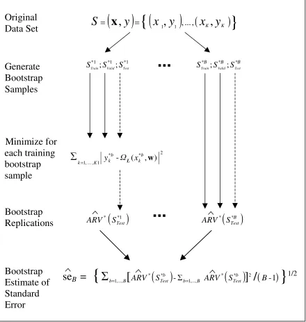
The bootstrapping approach as utilized in this study is illustrated in Figure 1. The idea
behind this approach is to generate many pseudo-replicates of the training, validation
and test sets, then re-estimating the model parameters w on each training bootstrap
sample, and testing the out-of-sample performance on the test bootstrap samples. In this
bootstrap world, the errors of forecast, and the errors in the parameter estimates, are
directly observable. The Monte-Carlo distribution of such errors can be used to
approximate the distribution of the unobservable errors in the real parameter estimates
and the real forecasts. This approximation is the bootstrap: it gives a measure of the
statistical uncertainty in the parameter estimates and the forecasts. Focus is laid in this
study on the performance of the forecasts measured in terms of ARV.
In more detail the approach may be described by the following steps: The details may
be a bit complicated, but the main idea is straightforward:
Step 1: Conduct three totally independent resampling operations in which
(i) B independent training bootstrap samples are generated, by randomly
sampling K1 times, with replacement, from the observed input-output
{
( * , * ),( * , * ),...,( * , * )}
* 1 1 2 2 1 1 b k b k b k b k b k b k bTrain x y x y x K y K
S = (7)
for k1, k2,..., kK1 a random sample of integers 1 through K1 < K and
b = 1,..., B [in this study: K=992, K1=480, B=376],
(ii) B independent validation bootstrap samples are formed, by randomly
sampling K2 times, with replacement, from the observed input-output
pairs S:
{
( * , * ),( * , * ),...,( * , * )}
* 2 2 2 2 1 1 b k b k b k b k b k b k bValid x y x y xK y K
S = (8)
for k1, k2,..., kK2 a random sample of integers 1 through K2 < K1 < K
and b = 1,..., B [in this study: K2=256],
(iii) B independent test bootstrap samples are formed, by randomly
sampling K3 times, with replacement, from the observed input-output
pairs S:
{
( * , * ),( * , * ),...,( * , * )}
* 3 3 2 2 1 1 b k b k b k b k b k b k bTest x y x y x K y K
S = (9)
for k1, k2,..., kK3 a random sample of integers 1 through K3 = K2 < K1 <
K and b = 1,..., B [in this study: K3=256],
Step 2: For each training bootstrap sample STrain*b (b=1,..., B) minimize
2 1 1 * * ) , (
∑
= − K k b k L b k xy Ω w (10)
with the differential evolution procedure. The training process is stopped when
) ( *
* b
Valid S
ARV defined by (6) starts to increase. This yields bootstrap parameter
estimates wˆ*b.
Step 3: Calculate the bootstrap ARV-Statistic of generalization performance,
) (
ˆ * *b
Test
S V R
pseudo-errors ARˆV*−ARˆV can be computed, and used to approximate the
distribution of the real errors ARˆV*−ARV . This approximation is the
bootstrap.
Step 4: The variability of ARˆV*(STest*b ) for b=1,..., B gives an estimate of the expected
accuracy of the model performance. Thus, estimate the standard error of the
generalization performance statistic by the sample standard deviation of the B
bootstrap replications:
(
)
21 1 2 * * * 1 / (.)] ˆ ) ( ˆ [ e ˆ s − − =
∑
= B b b TestB ARV S ARV B (11)
where
∑
= = B b b Test S V R A V R A 1 * * * ) ( ˆ (.)ˆ . (12)
Note that the name ’bootstrap’ refers to the use of the original sample pairs to generate
new data sets. The procedure requires to retrain the neural spatial interaction model B
times (see Step 2). Typically, the B is in the range 20≤ B≤200 (see Tibshirani 1996). Increasing B further does not bring a substantial reduction in variance (Efron and
Tibshirani 1993).
5. Data and Experimental Results
To demonstrate the bootstrapping approach, we use the Austrian telecommunication
flow data (see Fischer and Gopal 1994 for details). The data set was constructed from
three data sources: a (32, interregional telecommunication flow matrix, a (32,
32)-distance matrix, and gross regional products for the 32 telecommunication regions. We
have K = 992 input-output patterns. K1=480, K2=K3=256, and B=376. All inputs and
the target data were scaled to have zero mean and unit variance over the entire original
data set. In contrast to Fischer et al. (1999) we did not use a log-transformation of the
We use that model specification with J = 8 from the class ΩL(x, w) with one hidden
layer of logistic units and a linear output unit. The initial parameters were drawn at
random from an uniform distribution between -0.3 and 0.3. The differential evolution
method with κ=0.9 was used for the task of parameter estimation. All computations
were done on a DEC Alpha Cluster 350 MHz.
FIGURE 2 ABOUT HERE
Figure 2 shows the learning curves of a typical run, for STrain*b , SValid*b and STest*b in terms
of the ARV
(
STrain*b)
, ARV(
SValid*b)
and ARV( )
STest*b respectively. The term learning curve is used to characterize the as a function of iterations of the differential evolutionmethod. Figure 1(a) plots the ARV performance on the training bootstrap set, Figure
1(b) the ARV performance on the validation bootstrap set and Figure 1(c) the ARV
performance on the test bootstrap set. Note the clear increase of validation and test
errors after passing through minima, usually called overfitting or overtraining. At some
stage - in this specific run with a very small number of iterations around 70 - the model
extracts a feature of the training set that helps the testset, but hurts the validation set.
Note also that the minima of the validation set and the test set do not occur at the same
learning time. From each of these sets of learning curves, only a single number is used
for the subsequent analysis and comparisons in this paper: the ARV performance value
on the test set at that time that has the minimum of the validation set.
Several experiments were conducted to get a better statistical picture of model
performance measured in terms of out-of-sample performance, including the ability to
estimate the effect of the randomness of the splits of the data versus the randomness of
initial conditions of the spatial interaction model. The experiments involve a nested
iteration. At the ’outer loop’ training, validation and test bootstrap data sets are built up
one after another B times. The training sets are presented to the ’inner loop’ for random
parameter initialization of the spatial interaction model. At each pass through the outer
loop training, validation and test bootstrap samples are generated as independent draws
from S, B times. On each pass through the inner loop the d=41 individual weights of the
[-0.3, 0.3], B times, the model being re-estimated, and the ARV-statistic calculated on
the test sample.
TABLE 1 and FIGURE 3 ABOUT HERE
Table 1 along with Figure 3 summarize the results of a [degenerated bootstrap]
experiment, with B=1 and =376. The experiment serves to illustrate the impact of
parameter initialization on the out-of-sample performance of the neural spatial
interaction models. Figure 3 (b)-(f) shows the empirical density from 376 simulations
based upon B=1 and =376, while Figure 3(a) displays the empirical density from
B=376 bootstrap resamplings with =1. The fact that the width of the histograms (b)-(f)
tends to be smaller than the histogram (a) indicates that the randomness in network
model initialization generates less variability than the randomness in the splitting of the
data. Table 1 presents the out-of-sample model performance in terms of both the mean
of 376 simulations (column 1) and the standard deviation (column 2). The
Mann-Whitney U test statistic (column 3), a robust non-parametric test for the equality
between two independent distributions, provides evidence that the empirical densities
from 376 simulations based upon B=1 and 376 are significantly different from that
based upon B=376 bootstrap replicates and 1. The test statistic has a distribution that
is asymptotically normal with zero mean and unit variance under the null hypothesis
that the distributions are the same.
TABLE 2 and FIGURE 4 ABOUT HERE
Table 2 along with Figure 4 reports the results of a bootstrap experiment along with
B=376 and 1. This experiment serves to illustrate the impact of variations in training,
validation and test sets. In the simulation world of this experiment the standard
deviations of the 376 bootstrap replications are substantially less variable, but on the
whole larger than those appearing in the first experiment. This clearly indicates that the
randomness in the splitting of the data generates more variability than the randomness
in the network model initialization does. Figure 4 illustrates that the empirical densities
from the 376 bootstrap replications are relatively similar and not significantly different
6. Conclusions
This paper tried to combine bootstrap based statistical tests with neural spatial
interaction modelling to get a better statistical picture of forecast variability of the
model. Forecast variability can come from many sources. We focused on the noise due
to the data set resampling which may be termed sample noise and parameter noise
stemming from the choices in parameter initialization. Other noise sources, very
different in nature, such as errors-in-variables or model misspecification had been
outside of the scope of this paper. Utilizing the Austrian interregional
telecommunication traffic data and the differential evolution method [M=300, κ=0.9]
for solving the parameter estimation task for a fixed topology of the network model
[J=9] the study gave us important insights into the variability of forecast performance
over changes in training, validation and test samples, and parameter initialization. For
our example, most of the variability in forecast performance was clearly coming from
sample variation and not from variation in parameter initializations. This implies that it
is important not to over-interpret a model, estimated on one specific static split of the
data.
The bootstrap approach proved to be extremely useful in getting a clearer picture of
what might be real and what is noise. But it is important to keep in mind that each
bootstrap iteration requires a run of the differential evolution method on the training
bootstrap set. In very large real world problem contexts this computational burden may
become prohibitively large.
Finally, it is worth mentioning that there are several other computationally intensive
methods such as the jackknife and balanced repeated replications that are similar in
spirit to the bootstrap procedure but quite different in detail (see Efron and Tibshirani
1993 for more details). Each of these procedures generates ’pseudo-data’ sets from the
original data and assesses the actual variability of a statistic from its variability over all
the sets of pseudo-data. The procedures differ from the bootstrap and from one another
References
Bishop C M (1995) Neural networks for pattern recognition. Clarendon Press, Oxford
Efron B (1982): The jackknife, the bootstrap and other resampling plans. Philadelphia,
Society for Industrial and Applied Mathematics
Efron B, Tibshirani R (1991) Statistical data analysis in the computer age. Science 253:
390-394
Efron B, Tibshirani R (1993) An introduction to the bootstrap. Chapman and Hall, New
York
Fischer M M, Gopal S (1994) Artificial neural networks: A new approach to modelling
interregional telecommunciation flows. Journal of Regional Science 34(4):
503-527
Fischer M M, Hlavackova-Schindler K, Reismann M (1999) A global search procedure
for parameter estimation in neural spatial interaction modelling. Papers in
Regional Science 78: 119-134
Fischer, M M (1998) Computational neural networks: A new paradigm for spatial
analysis. Environment and Planning A 30 (10): 1873-1891
Hornik K, Stinchcombe M, White H (1989) Multilayer feedforward networks are
universal approximators. Neural Networks 2: 359-366
LeBaron B, Weigend A S (1998) A bootstrap evaluation of the effect of data splitting
on financial time series. IEEE Transactions on Neural Networks 9(1): 213-220
Mooney C Z, Duval R D (1993) Bootstrapping: A nonparametric approach to
statistical inference. Sage Publications, Newbury Park (CA)
Openshaw S (1993) Modelling spatial interaction using a neural net. In Fischer MM,
Nijkamp P (eds) Geographical information systems, spatial modelling, and policy
evaluation, pp. 147-164. Springer, Berlin
Openshaw S (1998) Neural network, genetic, and fuzzy logic models of spatial
Storn R, Price K (1997) Differential evolution – a simple and efficient heuristic for
global optimization over continuous spaces. Journal of Global
Optimization 11: 341-359
Tibshirani R (1996) A comparison of some error estimates for neural network models.
Neural Computation 8(1): 152-163
Weigend A S, Huberman B A, Rumelhart D E (1990) Predicting the future: A
Table 1. Variability of out-of-sample performance of the neural spatial interaction
model (2) with J=8, [M=300, κ=0.9] due to the randomness in parameter
initialization
Out-of-Sample Performance Mann-Whitney U Average Std.Dev. Test Statistic Data Samples A [B=1, =376] 0.2819 0.0888 11.72 [0.0000] Data Samples B [B=1, =376] 0.3016 0.1150 9.24 [0.0000] Data Samples C [B=1, =376] 0.4149 0.1015 -2.91 [0.0036] Data Samples D [B=1, =376] 0.4440 0.0574 -7.14 [0.0000] Data Samples E [B=1, =376] 0.5895 0.0514 -16.90 [0.0000] Bootstrap A as Benchmark [B=376, =1] 0.4009 0.1541 - -Average: Performance values [measured in terms of out-of-sample ARV] represent the mean of =376 simulations differing in the initial parameter values randomly chosen from (-0.3, 0.3) in the case of data samples A-E.
Std.Dev.: Performance values [measured in terms of out-of-sample ARV] represent the standard deviation of =376 simulations differing in the initial parameter values randomly chosen from (-0.3, 0.3) in the case of data samples A-E.
Table 2. Variability of out-of-sample performance of the neural spatial interaction
model (2) with J=8, [M=300, κ=0.9] due to sample variation
Out-of-Sample Performance Mann-Whitney U Average Std.Dev. Test Statistic Bootstrap A [B=376, =1] 0.4009 0.1541 - -Bootstrap B [B=376, =1] 0.3974 0.1479 0.27 [0.7896] Bootstrap C [B=376, =1] 0.4100 0.1595 -0.93 [0.3541] Bootstrap D [B=376, =1] 0.3920 0.1409 0.21 [0.8359] Bootstrap E [B=376, =1] 0.4064 0.1419 -1.17 [0.2410] Bootstrap F [B=376, =1] 0.4057 0.1539 -0.76 [0.4458] Average: Performance values [measured in terms of out-of-sample ARV] represent the mean of B=376 bootstrap replications with identical ( =1) parameter initializations randomly chosen from (-0.3, 0.3)
Std.Dev.: Performance values [measured in terms of out-of-sample ARV] represent the standard deviation of B=376 bootstrap replications with identical ( =1) parameter initializations randomly chosen from (-0.3, 0.3)
Figure 1. A diagram of the bootstrap procedure for estimating the standard error of
the generalization performance of neural spatial interaction models
Original
Data Set
Generate
Bootstrap
Samples
1 * 1 * 1 * ; ; Valid TestTrain S S
S
( ) (
y
x
y
)
(
x
Ky
K)
S
=x
,
= 1,
1 ,...,,
*B *B *B
Test Valid Train S S
S ; ;
2
1 , ... ,
1 - ( ,w)
b * k b * k K
k= y L x
Bootstrap
Replications
Bootstrap
Estimate of
Standard
Error
( )
*1 *Test
S
ARV ARV*
( )
STest*B( )
-( )
]
/
(
-1)
[
* 2,..., 1 *
,...,
1 ARV S ARV S B
*b Test B b *b Test B
b= =
...
...
Minimize for
each training
bootstrap
sample
{
}
1/2{
}
Figure 2. Learning curves of one specific neural spatial interaction model [J=8] and
parameter conditions [M=300, κ=0.9]. They show the performance versus
the learning time in terms of iterations: (a) the performance on a training
bootstrap set, (b) the performance on a validation bootstrap set, and (c) the
performance on a test bootstrap set.
(a) Training Set
Learning Time in Terms of Iterations
P e rf or m a nce I ndex A R V
0 200 400 600 800 1000
0. 2 0. 4 0. 6 0. 8 1. 0
(b) Validation Set
Learning Time in Terms of Iterations
P e rf or m a nce I ndex A R V
0 200 400 600 800 1000
0. 2 0. 4 0. 6 0. 8 1. 0
(c) Test Set
Learning Time in Terms of Iterations
P e rf or m ance I ndex A R V
0 200 400 600 800 1000
Figure 3. Histograms of out-of-sample performance [measured in terms of ARV] of
the neural spatial interaction model (2) with J=8 [M=300, κ=0.9]:
Variability due to the randomness in parameter initialization
0.0 0.2 0.4 0.6 0.8 1.0
0 2 04 06 0 8 0
(a) Data Samples A [B=1, b=376]
ARV
F
requenc
y
0.0 0.2 0.4 0.6 0.8 1.0
0 2 04 06 0 8 0
(c) Data Samples C [B=1, b=376]
ARV
F
requenc
y
0.0 0.2 0.4 0.6 0.8 1.0
0 2 04 06 0 8 0
(e) Data Samples E [B=1, b=376]
ARV
F
requenc
y
0.0 0.2 0.4 0.6 0.8 1.0
0 2 04 06 0 8 0
(b) Data Samples B [B=1, b=376]
ARV
F
requenc
y
0.0 0.2 0.4 0.6 0.8 1.0
0 2 04 06 0 8 0
(d) Data Samples D [B=1, b=376]
ARV
F
requenc
y
0.0 0.2 0.4 0.6 0.8 1.0
0 2 04 06 0 8 0
(f) Benchmark: Bootstrap A [B=376, b=1]
ARV
F
requenc
y
(a) Data Samples A [B=1, β=376] (b) Data Samples B [B=1, β=376]
(c) Data Samples C [B=1, β=376] (d) Data Samples D [B=1, β=376]
Figure 4. Histograms of out-of-sample performance [measured in terms of ARV] of
the neural spatial interaction model (2) with J=8 [M=300, κ=0.9]:
Variability due to the randomness in data resampling
0.0 0.2 0.4 0.6 0.8 1.0
0 2 04 06 0 8 0
Bootstrap A [B=376, b=1]
ARV
F
requenc
y
0.0 0.2 0.4 0.6 0.8 1.0
0 2 04 06 0 8 0
Bootstrap C [B=376, b=1]
ARV
F
requenc
y
0.0 0.2 0.4 0.6 0.8 1.0
0 2 04 06 0 8 0
Bootstrap E [B=376, b=1]
ARV
F
requenc
y
0.0 0.2 0.4 0.6 0.8 1.0
0 2 04 06 0 8 0
Bootstrap B [B=376, b=1]
ARV
F
requenc
y
0.0 0.2 0.4 0.6 0.8 1.0
0 2 04 06 0 8 0
Bootstrap D [B=376, b=1]
ARV
F
requenc
y
0.0 0.2 0.4 0.6 0.8 1.0
0 2 04 06 0 8 0
Bootstrap F [B=376, b=1]
ARV
F
requenc
y
(a) Bootstrap A [B=376, β=1] (b) Bootstrap B [B=376, β=1]
(c) Bootstrap C [B=376, β=1] (d) Bootstrap D [B=376, β=1]


![Figure 2.Learning curves of one specific neural spatial interaction model [J=8] and](https://thumb-us.123doks.com/thumbv2/123dok_us/8112592.791495/23.595.93.501.200.515/figure-learning-curves-specific-neural-spatial-interaction-model.webp)
![Figure 3.Histograms of out-of-sample performance [measured in terms of ARV] of](https://thumb-us.123doks.com/thumbv2/123dok_us/8112592.791495/24.595.93.503.179.472/figure-histograms-sample-performance-measured-terms-arv.webp)
![Figure 4.Histograms of out-of-sample performance [measured in terms of ARV] of](https://thumb-us.123doks.com/thumbv2/123dok_us/8112592.791495/25.595.93.501.184.470/figure-histograms-sample-performance-measured-terms-arv.webp)
