A Scoring Method for the Clustering of Nucleic
Acid Sequences
Barileé Barisi Baridam
Department of Computer Science University of Pretoria
South Africa
ABSTRACT
The clustering of biological sequence data i s a significant task for biologists. The reason is that sequence clustering assists molecular biologists to group sequences based on the ancestral traits or hereditary information that are hidden in sequences. To accomplish the similarity detection and clustering tasks, several clustering algorithms, similarity and d i s t an c e measures have b e e n proposed. Most of these algorithms a n d si milarity measures manifest some form of inefficiency in the detection of sequences based on their structural similarity as was observed in the cou r s e of this study. In this paper, the codon -based scoring method (COBASM) is developed to handle this inefficiency. COBASM employs the codon principle, by the application of triplet nucleotides, in the clustering of nucleic acid sequences. The results obtained show that COBASM is able to produce compact and well- separated clusters based on the structural similarity of sequences.
General Terms
Clustering, algorithm, similarity measure, sequences.
Keywords
Codon, scoring method, similarity measure, clustering
1.
INTRODUCTION
In computational biology, clustering goes beyond a mere statistical tool for information retrieval. In sequence clustering, it aims at revealing the genetic information of participating sequences. Cluster analysis helps in the determination of gene families and the establishment of implicit links between them. Clustering of biological sequence data presents a great challenge to the computing society as well as to biologists. This challenge arises from the fact that conventional similarity measures exhibit difficulty in detecting structural similarities among sequences, and that sequences cannot be easily clustered by the application of conventional distance or similarity measures that are commonly applied to numeric data sets. This is so because nucleic acids sequences are never represented numerically. Nucleic acid sequences are represented by symbols. Also, string edit distance algorithms [1] employed in string comparisons and string similarity searches are mostly not suitable in biological sequence data clustering [2]. This is basically because, as stated above, the structural nature of biological sequences makes string edit distance [1] not appropriate. For example, the edit between the strings
(sequences) CCCCCCCGGGGGGG and
GGGGGGGCCCCCCC showsthere is no similarity between the strings. However, looking at the strings biologically, there is an element of structural similarity which the edit distance neglects. The application of multiple sequence alignment is
Because structural similarity is a major issue in biological sequence analysis, it becomes very important to design a similarity measure (scoring method) that will consider such, without the introduction sequence alignment.
1.1
The Case of Sequence Homology
Similar biological sequences, nucleotides or amino acids are often derived from the same ancestral sequence and are therefore expected to share common structure and function even when the sequences are from different organisms. These sequences, which are very similar, are called homologues. It is believed, for example, that if the sequences are about 100 nucleotides long (or 100 amino acids long for proteins), they may be considered homologous if 70 percent of the nucleotides (or 25 percent of amino acids) are identical [3]. Where the percentage values are less than 70 (or 25), as the case may be, it is believed that the twilight zone, where the meaning of the observed similarity is doubtful and homology (similarity due to common evolutionary history) or non-homology is never guaranteed, is reached. The non-homology concept is utilized in the codon-based scoring method,
COBASM1.
2.
CLUSTERING AND SIMILARITY
SEARCH PROBLEMS
The successful application of the average linkage hierarchical clustering algorithm for the expression data of budding yeast Saccharomyces cerevisiae and the reaction of human fibroblasts to serum by Eisen et al [4] heralded the application of cluster analysis in the grouping of functionally similar genes [5]. In particular, hierarchical clustering has been used to organize genes into a hierarchical dendrogram on the basis of genes expression across multiple growth conditions. Cluster analysis, for example in gene expression data, has two aspects: clustering genes [6], [7], and clustering tissues or experiments [8], [9]. The clustering of gene expression data in these categories marked a significant breakthrough in the application of cluster analysis in the clustering of biological data.
Other fields where clustering have been applied are in biotechnology, concept decomposition for large sparse data [10], high dimensional and distributed data [11], [12], [13], [14], [15], spatial data mining [16], [17], intrusion detection systems [18], imaging [19], circuit partitioning in VLSI design [20], and computer vision [21]. Clustering is also applied in outliers detection or in finding unusual data objects [22].Several clustering methods and algorithms have been proposed by researchers, yet there is still a growing concern about the quality of clusters generated by clustering
1
algorithms. Although there exist sequence clustering algorithms, majority of them are generally string-based without the consideration of biological sequences. Among the clustering algorithms and methods proposed in biological sciences are: (1) CHAMELEON - which performs clustering through measuring the sim- ilarity of clusters based on a dynamic model [23]; (2) FOLDALIGNM - developed by Elfar Torarinsson et al [24], makes use of multiple alignment in the clustering of RNA sequences; (3) AMICA - a metric incremental clustering algorithm, which allows the formulation of an incremental clustering of nominal data [25]; (4) the HMM-Clustering algorithm [26], [27]; (5) WARLUS - a similarity retrieval algorithm for image databases [28]; (6) Query-Dependent Banding (QDB) algorithm for RNA similarity searches [29]; (7) KMS for multiple DNA sequence approximate matching [30]; (8) CLARA [17]; (9) CLARANS [17]; (10) MetricMap [31]; (11) QTClust algorithm employed in the identification and analysis of co-expressed genes [32]; (12) the coupled two-way clustering analysis algorithm for the clustering of gene microarray data [33]; and (13) the 4C algorithm [34]. Among the list of clustering algorithms developed for biological data clustering are those of Xing and Karp [11] and Zhao and Zaki [35]. Xing and Karp [11] developed the CLIFF algorithm for the clustering of high- dimensional microarray data via iterative feature filtering. Zhao and Zaki [35] introduced the TRICLUSTER algorithm for the mining of coherent clusters in 3D microarray data.
3.
THE CODON -BASED SCORING
METHOD
The codon-based scoring method (COBASM) introduced in this paper employs the codon arrangement as depicted on the codon (or genetic code) table. It considers grouping the constituent bases into three, based on their codon arrangements. The reason for considering groups of three bases is because it is biologically significant and meaningful to consider a triplet of bases as it is useful in the formation of amino acids. Blocks of three similar nucleotides are used to capture the codon arrangement as indicated on the codon (genetic code) table in the formation of the twenty amino acids found in protein. Blocks of two, four or five will not give a meaningful interpretation of the concept being investigated. For example, the pairs, GC and AT, are the only compatible base pairs when considering the pairing of DNA bases in the formation of DNA‟s double helix. Pairing A and C are incompatible and will yield no significant result. This is because the pair between A and C are incompatible and chemically unstable, owing to the loss of the hydrogen bond formed within the base pair. This fact renders the choice of blocks of two, four or five irrelevant and biologically insignificant. Therefore, basing the underlying concept upon a combination of bases other than the codon concept presented in this paper is not biological and as thus, will produce no significant result.
COBASM takes an entire source sequence and compares each character with the target sequence as does the Levenshtein distance [1], but with some major improvements. The scoring method proposed in this paper assigns a score of 1 to each corresponding pair of nucleotides that are similar, and 0 to
dissimilar pairs. An additional 1 is given for consecutive blocks of three pairs of similar nucleotides. The codon-based similarity is explained as follows:
Consider two sequences su and sv as source and target
sequences, respectively. In the first instance, sequences of equal length were considered. Each successive block of bases in the source sequence is placed in adjacent blocks in the target sequence. Corresponding sequences are scored accordingly. This method is similar to the method employed in the detection of motif [36]. Secondarily, a situation where n
(length of su ) and m (length of sv ) are unequal, i.e. n ≠ m, the
sequences are treated as follows:
A wise search is conducted among the sequences. A pair-wise search in this case involves the positioning of individual characters in the source sequence against the target sequence until their last characters meet. The movement (pair-wise comparison) along the source sequence is done (n − m) times. This has also been described in the pseudo-code represented by Figure 3.
From the above, it is clear that d( su , sv ) = d(sv , su ) when n =
m, and when n ≠ m, d( su , sv ) = d(sv , su ) indicating
symmetricality. The pseudo-code for the case n = m and n < m is also presented. For n > m, d(sv , su ) is used instead of d(
su , sv ), see Baridam [37] for the detailed description of the
implementation.
Captions should be Times New Roman 9-point bold. They should be numbered (e.g., “Table 1” or “Figure 2”), please note that the word for Table and Figure are spelled out. Figure‟s captions should be centered beneath the image or picture, and Table captions should be centered above the table body.
3.1
Implementation of COBASM
Recall that, nucleic acid sequences are considered homologous (similar) when at least 70% nucleotides are identical. We now explain how this is implemented in the clustering based on COBASM.
Let su and sv be the source and target sequence, respectively.
The highest match count occurs if su and sv are identical (and
of the same length n). According to the definition of COBASM, the highest matching count is calculated as
1
3
2
3
1
n
n
i
i
n i
(1)
There can be any level of match count (including zero) between the source and the target. The 70% homology level is now calculated from equation (1) using:
1
15
7
1
3
2
.
100
70
n
n
n
n
Fig 1: A pseudo-code for the codon-based scoring method
For any two sequences su and sv , the total match (similarity) count, d(su , sv ), is calculated using COBASM as stated, and they are considered similar if
d(su , sv ) ≥ Hs (3)
holds. The COBASM-based clustering algorithm (or simply COBASM algorithm) employs the codon-based similarity measure in the clustering of biological sequences based on the homology principle.
To describe how a cluster is formed and, in particular, how a sequence is assigned to a cluster, consider the data set
S = {s1 , s2 , · · · , su , · · · , sv , · · · sN } (4) of biological sequences si , i = 1, 2, • • • , N . N is the total number sequences in the data set. Any two sequences su , sv ∈
S may have different lengths. The COBASM algorithm selects an element, say su , of S at random and considers this as the
centroid of the first cluster.
The target sequences, sv, are then considered, one after the
other, from the unclustered sequences to form the first cluster using the similarity measure COBASM. The COBASM algorithm then selects the second centroid, at random, from the remaining unclustered sequences to form the second cluster, and the process continues in this way until all sequences are clustered. The random selection of centroids in the COBASM clustering algorithm is very useful for simulation purposes.
Although COBASM can be applied in the clustering of other strings or sequence data, it is particularly useful in the clustering of biological sequences, and mostly suitable for
handling the structural similarities of sequences where the participating sequences are of unequal lengths. This implies that COBASM is very efficient working with multi-dimensional problems.
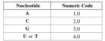
Table 1. The nucleic coding scheme for numeric-based distance measures
Nucleotide Numeric Code
A 1.0
C 2.0
G 3.0
U or T 4.0
3.2
Applying other similarity measures
For comparison purpose, three similarity measures were used in the clustering of selected biological data sets defined by (4). They are (a) Manhattan, (b) Euclidean and (c) Edit distances (ED). For the distance (similarity) measures Manhattan and Euclidean, the conversion of nucleic acid symbols to numeric is done, as presented in Table 1, and presented in an n-dimensional plane.The Levenshtein (edit) distance [1] is the maximum number of edit operations (insertions, deletions or substitutions) needed to transform one string to another. The edit distance compares the similarity between su and sv and implements (3) by reversing the inequality sign, i.e. su and sv are treated similar if d(su , sv ) ≤ 30% of total number of edits. The Euclidean and Manhattan measures are given by
[image:3.595.338.512.498.567.2]Initialize S_1 and S_2 for |S_1|: i= 1 to n do
for |S_2|: j= 1 to m do //determine the length of the longest //sequence if sequences are unaligned //or unequal.
if n < m then //if length of sequences are not equal //do pattern-element-search Compare s_1[i] with s_2[j],s_2[j+1],...,s_2[m-n] and s_1[i+1] with s_2[j+1],s_2[j+2],...,s_2[m-n+1]
if s_1[i] = s_2[j] then score = 1
else score = 0 endif
endif
if n = m then //examine each character of S_1 and S_2 if s_1[i] = s_2[j] then
score = 1 else score = 0 endif
endif
//split sequences S_1 and S_2 (including //gaps if aligned) into blocks of three //bases each and compare adjacent blocks. for i,j >= 0 do //total block-match.
if s_1[i+1,i+2,i+3] = s_2[j+1,j+2,j+3] then score = score+1
else
return score endif
n
i
u
i
v
i
d
s
us
vs
s
1
,
2
(5)
and
ni
v u v
u
s
s
s
s
i id
1
,
, (6)respectively. These two measures treat su and sv similar if d(su , sv ) ≤ λ, where λ is a certain percentage (e.g. 20%) of an average length. The average length is based on a sample taken from S. The length of a vector si ∈ S is calculated as d(si , 0) using (5) and (6) for Euclidean and Manhattan measures, respectively; the zero in d(si , 0) is the zero vector [37].
4.
MEASURE OF QUALITY
To assess the quality of clusters formed under the four distance measures, three measurement quantities were used. These are the quantization error function [19], and the intra and inter cluster distance functions. The quantization error is a measurement of the quality of the clusters formed. To determine the compactness and separability of the clusters, the intra and inter-cluster distance functions were employed.
The quantization error (Qe) function is defined as
Km i
m i m
e
S
d
K
m
C
s
S
Q
1 1
,
1
1
(7)
where Sm is the mth cluster, si is the i th
sequence in cluster Sm, Cm is the centroid of Sm, |Sm| is the number of sequences in Sm
and K is the number of clusters formed for the clustering problem. The inner average in (7) is taken over each cluster and the outer average is taken over the total number of clusters, K. The distance d(si, Cm) under different similarity
measures, between the ith sequence of the mth cluster and the centroid of the cluster is calculated as discussed earlier.
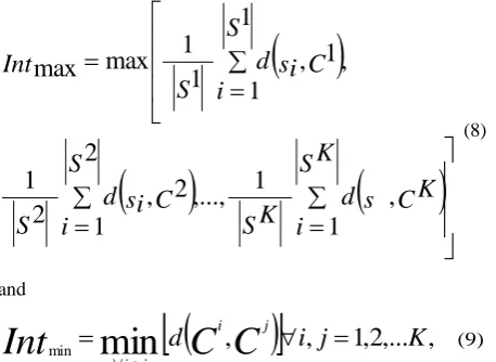
The intra and inter-cluster distances are measured by calculating the maximum and minimum distance within and between the clusters, respectively [19], and are given as
S K
i
C K
s
d
S K
S
i
C
si
d
S
S
i
C
si
d
S
Int
1
,
1
,...,
2
1
2
,
2
1
,
1
1
1
,
1
1
max
max
(8)
and
,
,
1
,
2
,...
,
min
min
d
C
C
i
j
K
Int
i jj i
(9)
where K is the total number of clusters.
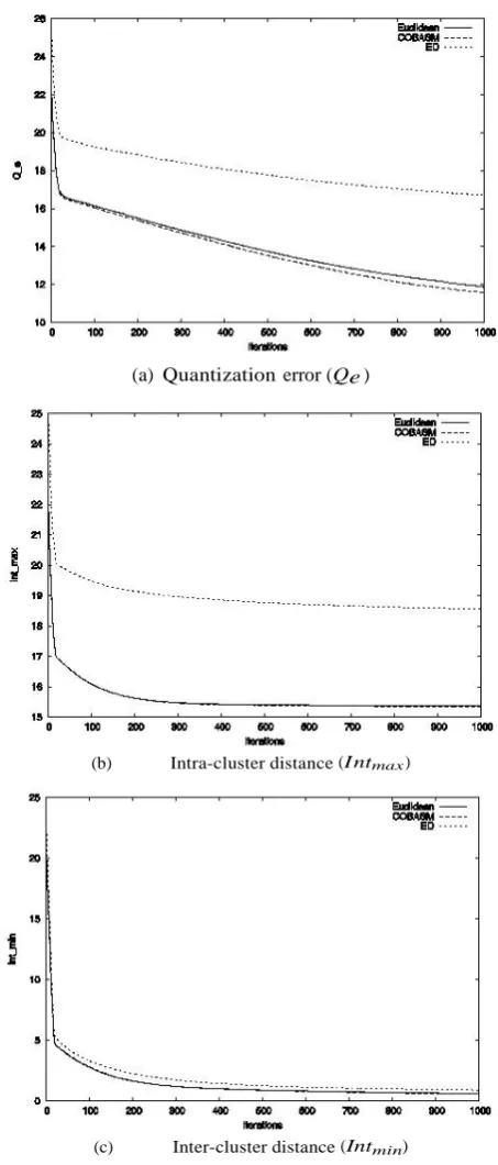
(a) Quantization error (Qe )
(b) Intra-cluster distance (I ntmax )
[image:4.595.55.284.536.703.2](c) Inter-cluster distance (Intmin )
Figure 2. Graphical representation of the performance of the distance measures on Dataset 3
5.
EXPERIMENTAL RESULTS
Six data sets were used, namely emblFasta Rickettsia typhi str. RNA sequences with Accession Number AE017197 from Wilmington Complete Genome of 1111500 nucleotides, Homo sapiens‟ melanatonic melanoma DNA sequences, mRNA bos taurus sequences from Genetic Sequence Databank with Accession Number BE484664 obtained from the work of Sonstegard, et al [38], and DNA dental sequences from Department of Micro-biology, University of Pretoria, South Africa.
Dataset 1: 500 Rickettsia typhi str. RNA sequences consisting of 30000 nucleotides.
Dataset 2: 200 Rickettsia typhi str. RNA sequences consisting of 12000 nucleotides.
Dataset 3: 100 Rickettsia typhi str. RNA sequences consisting of 6000 nucleotides.
Dataset 4: 31 DNA dental sequences of varying lengths consisting of approximately 12550 nucleotides.
Dataset 5: 20 Homo sapiens’ melanatonic melanoma DNA sequences of varying lengths and a total of 15658 nucleotides with the longest sequence having 1471, and the shortest 134 nucleotides long.
Dataset 6: 141 mRNA bos taurus sequences of 29718 nucleotides with the longest sequence having 508, and the shortest 198 nucleotides long. Accession date: June 15, 2008.
The results obtained (Table 2) are products of experiments performed with 30 simulations over 1000 iterations. The results in Table 2 summarizes the performance of the various distance measures. On the average, COBASM demonstrates an overall best performance over the rest of the distance measures as observed from the table. In particular, on Dataset 6 COBASM‟s performance is considerably significant. The
Qe, Intmaxand Intmin values obtained by COBASM on Dataset
6 are 11.5746, 15.3420 and 0.5963, respectively.
6.
PERFORMANCE EVALUATION
The quality measurements of the obtained clusters using four distance measures are summarized in Table 2. The results presented are based on experiments performed with 30 simulations over 1000 iterations. The format of data in Table 2 is „mean value ± the standard deviation‟. Table 2 shows that, on the average, COBASM demonstrates an overall best performance over the rest of the distance measures. In particular, on Dataset 6 COBASM‟s performance is considerably significant. The Qe , Intmax and Intmin values for
this case are better than the values obtained by the other measures.
6.1
Graphical representation
Graphical representation of the performance of the distance measures (Euclidean, edit and COBASM) on Dataset 6 and Datasets 1, 2 and 3 (the Rickettsia typhi str. datasets) are given in this section. The performance of the Manhattan distance measure is poorer than all the other distance measures, and so it is not captured on the graphs.
The performance of COBASM on Dataset 3 is measured with the edit distance and the Euclidean distance measures. The result of performance with „Dataset 3 - emblfasta100‟ (so-called because of the presence of 100 sequences in this case) - is presented in Figure 2. From Figure 2(b and c) COBASM
produces a more compact cluster with the data set in comparison to the other distance measures. On the average, a better clustering result is achieved with COBASM.
(a) Quantization error (Qe )
(b) Intra-cluster distance (I ntmax )
[image:5.595.314.541.106.637.2](c) Inter-cluster distance (Intmin)
The graphs in Figure 3 show the performance of COBASM on Dataset 6 data set as compared with the other distance measures. The graphs indicate that a more compact and separated clusters are produced with COBASM on the data set than with other distance measures.
6.2
Statistical analysis of results
The statistical test tool applied in this analysis is the Analysis of Variance (ANOVA) Test [39]. The ANOVA test was used instead of the Friedman‟s Test [39]2 to compare observations among the data distributions be- cause of the nature of the data samples collected. Besides, ANOVA is useful in comparing a distribution of more than two means. It is also helpful because it possesses a certain advantage over a two-sample t-test which has an increased chance of committing a Type I error3 . Type I error is one of two types of statistical hypothesis testing errors that could be committed. A Type I error is the assumption that a null hypothesis4 should be rejected when in actual fact should be accepted as true. In clustering, this type of error is referred to as false negative. The inverse is a Type II error (false positive) - a situation where a null hypothesis is accepted despite being false.
The statistical results obtained using 30 simulations are presented in Tables 3 and 4, respectively for Intmaxand Intmin .
Both tables show that the degree of freedom (df) is 3, and the significance value (p value) of .03 (3%). This indicates that the results obtained were not due to chance. Statistically, the p
value should be equal or less than 5% (0.05) to claim that the relationship is truly significant. It is safe, from the tables, to conclude that the results obtained are mathematically significant.
Among the distance measures employed in the experiments the edit distance is the only distance measure that operates purely on string datasets. Euclidean and Manhattan distance measures are based on numeric values (recall that conversion has been done on the datasets, see Table 1). Tables 3 and 4 show that COBASM performs better than the rest of the distance measures. COBASM is now compared with edit
2
http://www.texasoft.com/tutorial-friedmans-test.html
3
http://en.wikipedia.org/wiki/Analysis of variance
4
A null hypothesis is a hypothesis under investigation that should be either nullified or not, based on the result of the test.
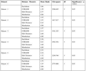
distance. Note that this comparison is particularly important since the edit distance is a string-based distance measure. Table 3 shows that, out of the six data sets used, COBASM‟s performance on five of the data sets is better than the edit distance.
COBASM‟s performance on Dataset 2 and Dataset 6 is of high significance with a mean ranking of 1.10 and 1.15, respectively. The results from Table 3 show that COBASM produces compact clusters than the rest of the distance measures. Out of the remaining three distance measures Manhattan‟s performance is generally poor.
The statistical analysis of the inter-cluster distance also provides promising results with COBASM. The mean ranking in Table 4 shows that the performance of COBASM on four of the six datasets is better than the other distance measures except on Dataset 2 and Dataset 6 where it has the same value with the Euclidean distance. Best results were obtained in comparison with edit distance on Datasets 1, 2 and 6 with values of 1.39, 1.93 and 1.25, respectively. The results show that COBASM produces well-separated clusters in comparison with the rest distance measures.
7.
CONCLUSION
This paper investigated the performance of the codon- based scoring method (similarity measure) alongside other distance measures in the clustering of nucleic acid sequences. The performances of three distance measures were examined alongside COBASM, namely Euclidean distance, Edit distance, and Manhattan distance, as they were applied in the clustering of high-dimensional problems. The application of codon in determining similarity among sequences as employed by COBASM was found to be better than these measures with respect to the determination of structural similarity, compactness and separability of the formed clusters. The application of COBASM to clustering biological sequences that are multi-dimensional was also done as seen from the nature of the data sets used.
Further research will involve the application of COBASM in the clustering of amino acids (protein) sequences and the implementation of COBASM alongside other existing string-based algorithms in the clustering of high/multi-dimensional data sets.
Table 2. Results from clustering with different distance measures
Distance Measures
Euclidean COBASM ED Manhattan
Problem Qe I ntmax I ntmin Qe I ntmax I ntmin Qe I ntmax I ntmin Qe I ntmax I ntmin
Dataset 1 8.6878± 0.3188 9.6209± 0.0411 0.0090± 0.0063 8.7365± 0.3940 9.6029± 0.0245 0.0086± 0.0069 8.7609± 0.3188 9.6104± 0.0301 0.0130± 0.0184 65.9062± 0.5783 64.9062± 0.1822 0.2768± 0.2968 Dataset 2 6.6618±
0.6143 9.5058± 0.0378 0.0088± 0.0042 6.9991± 0.4767 9.4943± 0.0403 0.0082± 0.0115 6.8485± 0.5189 9.5001± 0.0451 0.0071± 0.0072 60.7123± 1.0287 61.9791± 0.3216 0.2546± 0.2301 Dataset 3 5.7904±
0.5111 9.3149± 0.1213 0.0063± 0.0038 6.7359± 0.8771 9.6685± 0.0518 0.0123± 0.0179 7.4153± 1.2095 9.6590± 0.0558 0.0091± 0.0085 61.6671± 2.1160 63.7151± 0.5032 0.3718± 0.3699 Dataset 4 11.6696±
1.7625 12.9636± 0.9281 0.8272± 0.0906 12.1749± 1.5456 12.7128± 0.8456 0.8868± 0.1214 12.4180± 1.6634 12.5125± 0.6741 0.8215± 0.1235 152.4258± 15.1887 153.0170± 8.1400 13.3112± 2.0740 Dataset 5 7.1376±
1.0931 11.8205± 0.2710 0.2610± 0.0813 6.9292± 1.1531 11.8411± 0.3338 0.2666± 0.0924 6.8071± 0.9314 11.8964± 0.2575 0.2758± 0.0920 78.4570± 9.3383 109.3385± 9.0357 3.5257± 1.0425 Dataset 6 11.8744±
Table 3. Statistical results based on Intra-cluster distance, Intmax
Table 4. Statistical results based on Inter-cluster distance, Intmin
Dataset Distance Measure Mean Rank Chi-square df Significance (p value) Dataset 1
Euclidean COBASM Edit Distance Manhattan
1.84 1.39 2.77 4.00
2386.645 3 0.03
Dataset 2
Euclidean COBASM Edit Distance Manhattan
1.93 1.93 2.14 4.00
1817.917 3 0.03
Dataset 3
Euclidean COBASM Edit Distance Manhattan
1.27 2.13 2.60 4.00
2341.103 3 0.03
Dataset 4
Euclidean COBASM Edit Distance Manhattan
2.28 2.63 1.09 4.00
2581.036 3 0.03
Dataset 5
Euclidean COBASM Edit Distance Manhattan
2.52 2.16 1.32 4.00
2258.798 3 0.03
Dataset 6
Euclidean COBASM Edit Distance Manhattan
1.75 1.25 3.00 4.00
2775.000 3 0.03
Dataset Distance Measure Mean Rank Chi-square df Significance (p value) Dataset 1
Euclidean COBASM Edit Distance Manhattan
3.00 1.43 1.57 4.00
2703.832 3 0.03
Dataset 2
Euclidean COBASM Edit Distance Manhattan
2.16 1.10 2.75 4.00
2637.239 3 0.03
Dataset 3
Euclidean COBASM Edit Distance Manhattan
1.00 2.98 2.02 4.00
2974.181 3 0.03
Dataset 4
Euclidean COBASM Edit Distance Manhattan
2.80 1.37 1.83 4.00
2441.891 3 0.03
Dataset 5
Euclidean COBASM Edit Distance Manhattan
1.16 2.23 2.61 4.00
2471.872 3 0.03
Dataset 6
Euclidean COBASM Edit Distance Manhattan
1.85 1.15 3.00 4.00
[image:7.595.121.477.428.721.2]8.
REFERENCES
[1] V. I. Levenshtein, 1965. “Binary codes capable of correcting deletions, insertions, and reversals,” Doklady Akademii Nauk SSSR, vol. 163, no. 4, pp. 845–848.
[2] J. Yang and W. Wang, 2003. “CLUSEQ: efficient and effective sequence clustering,” in Proceeding of 19th International Conference Data Engineering, pp. 101– 1125.
[3] J. Claverie and C. Notredame, 2007. Bioinformatics for dummies, 2nd ed. Indiana: Wiley.
[4] M. Eisen, P. Spellman, P. Brown, and D. Botstein, 1998. “Cluster analysis and display of genome-wide expression patterns,” in Proceedings National Academy of Science, USA, vol. 95, pp. 14 863–14 868.
[5] R. Xu and D. Wunsch II, 2005. “Survey of clustering algorithms,” IEEE Transactions on Neural Networks, vol. 16, no. 3, pp. 601–614.
[6] A. Ben-Dor, R. Shamir, and Z. Yakhini, 2005. “Clustering gene expression patterns,” Journal of Computational Biology, vol. 6, no. 3/4.
[7] R. Sharan and R. Shamir, 2000. “CLICK: A clustering algorithm with applications to gene expression analysis,” in Proceedings of International Conference on Intelligent Systems and Molecular Biology, vol. 8, pp. 307–316.
[8] G. Getz, H. Gal, I. Kela, D. A. Notterman, and E. Domany, 2003. “Coupled two-way clustering analysis of breast cancer and colon cancer gene expression data,” Bioinformatics, vol. 19, no. 9, pp. 1079–1089.
[9] G. Getz, E. Levine, E. Domany, and M. Q. Zhang, 2000. “Super- parametric clustering of yeast gene expression profiles,” Physica A, vol. 279, pp. 457–464.
[10]I. S. Dhillon and D. S. Modha, 2001. “Concept decompositions for large sparse text data using clustering,” Machine Learning, vol. 42, pp. 143–175. [11]E. P. Xing and R. M. Karp, 2001. “CLIFF: Clustering of
high-dimensional microarray data via iterative feature filtering using normalized cuts,” Bioinformatics, vol. 17, no. 1, pp. s306–315.
[12]J. Liu and W. Wang, 2003. “OP-cluster: Clustering by tendency in high dimensional space,” in Proceedings of the Third IEEE International Conference on Data Mining.
[13]C. C. Aggarwal and P. S. Yu, 2000. “Finding generalized projected clusters in high dimensional spaces,” in ACM SIGMOD, pp. 70–81.
[14]R. Agrawal, J. E. Gehrke, D. Gunopulos, and P. Raghavan, 1998. “Automatic subspace clustering of high dimensional data for data mining applications,” in ACM SIGMOD.
[15]T. Li, S. Zhu, and M. Ogihara, 2003. “Algorithms for clustering high dimensional and distributed data,” Intelligent Data Analysis, vol. 7, no. 4, pp. 305–326.
[16]P. Berkhin, 2002. “Survey of clustering data mining techniques,” Accrue Software, Inc., San Jose, California,
Tech. Rep. 4, available online:
www.citeseer.nj.nec.com/berkhin02survey.html.
[17]R. Ng and J. Han, 2004. “CLARANS: A method for clustering objects for spatial data mining,” IEEE Transaction on Knowledge and Data Engineering, vol. 14, no. 5, pp. 1003–1016.
[18]V. Nikulin, 2006. “Weighted threshold-based clustering for intrusion detection system,” International Journal of Computational Intelligence and Applications, vol. 6, no. 1, pp. 31–19.
[19]M. G. H. Omran, 2004. “Particle swarm optimization methods for pattern recognition and image processing,” PhD thesis, University of Pretoria, Faculty of Engineering, Built Environment and Information Technology, Department of Computer Science.
[20]J. Cong and M. Smith. 1993. “A parallel bottom-up clustering algorithm with applications to circuit partitioning in VLSI design,” in Proceed- ings of the 30th ACM/IEEE Design Automation Conference, pp. 755– 760.
[21]H. Frigui and R. Krishnapuram. 1999. “A robust competitive clustering algorithm with applications in computer vision,” in IEEE Trans- actions on Pattern Analysis and Machine Intelligence, vol. 21, pp. 450–465.
[22]S. J. Devlin, R. Gnanadesikan, and J. R. Kettenring. 1975. “Robust estimation and outlier detection with correlation coefficients,” Biometrika, vol. 62, no. 3, pp. 531–545.
[23]G. Karypis, E. Han, and V. Kumar. 1999. “CHAMELEON: A hierarchical clustering algorithm using dynamic modeling,” IEEE Transaction on Computers, vol. 32, no. 8, pp. 68–75.
[24]E. Torarinsson, J. H. Havgaard, and J. Gorodkin. 2007. “Multiple structure alignment and clustering of RNA sequences,” Bioinformatics, vol. 23, no. 8, pp. 926–932. [25]D. Simovici, N. Singla, and M. Kuperberg. 2004.
“Metric incremental clustering of nominal data,” in Proceedings of the Fourth IEEE International Conference on Data Mining (ICDM‟04), vol. 00, pp. 523–526.
[26]P. Smyth. 1997. “Clustering sequences with hidden markov models,” Advances in Neural Information Processing Systems, vol. 648.
[27]F. Porikli. 2004. “Clustering variable length sequences by eigenvector decomposition using HMM,” Springer, vol. 3138.
[28]A. Natsev, R. Rastogi, and K. Shim. 2004. “WALRUS: A similarity retrieval algorithm for image databases,” IEEE Transaction on Knowledge and Data Engineering, vol. 16, no. 3, pp. 301–316.
[29]E. P. Nawrocki and S. R. Eddy. 2007. “Query-dependent banding (QDB) for faster RNA similarity searches,” PLOS Computational Biology, vol. 3, no. 3, pp. 0540– 0554.
[30]K. M. Kaplan and J. J. Kaplan. 2004. “Multiple DNA sequence approximate matching,” in Proceedings of the IEEE Symposium on Computational Intelligence in Bioinformatics and Computational Biology, pp. 79–86.
[31]X. Wang, J. T. Wang, K. Lin, D. Shasha, B. A. Shapiro, and K. Zhang. 2000. “An index structure for data mining and clustering,” Knowledge and Information Systems, vol. 2, no. 2, pp. 161–184.
[32]L. J. Heyer, S. Kruglyak, and S. Yooseph. 1999. “Exploring expression data: Identification and analysis of coexpressed genes,” Genome Research, vol. 9, pp. 1106– 1115.
Proceedings of National Academy of Science, USA, vol. 97, pp. 12 079–12 084.
[34]C. Bohm, K. Kailing, P. Kroger, and A. Zimek. 2004. “Computing clusters of correlation connected objects,” in ACM SIGMOD Conference.
[35]L. Zhao and M. Zaki. 2005. “TRICLUSTER: An effective algorithm for mining coherent clusters in 3d microarray data,” in ACM SIGMOD Conference.
[36]B. B. Baridam and O. Owolabi. 2010. “Conceptual clustering of RNA sequences with the codon usage model,” Global Journal of Computer Science and Technology, vol. 10, no. 8, pp. 41–45.
[37]B. B. Baridam. 2010. “Optimization techniques for the clustering of nucleic acids sequences,” PhD thesis, University of Pretoria.
[38]T. Sonstegard, A. V. Capuco, J. White, C. P. Van Tastell, E. E. Connor, J. Cho, R. Sultana, L. Shade, J. E. Wray, K. D. Wells, and J. Quackenbush. 2002. “Analysis of bovine mammary gland EST and functional annotation of the Bos Taurus gene index,” Mammary Genome, vol. 13, no. 7, pp. 373–379.