Performance of profiled single noise barriers covered with quadratic residue diffusers

Performance of profiled single noise 

barriers covered with quadratic residue 

diffusers

Monazzam, M and Lam, YW

http://dx.doi.org/10.1016/j.apacoust.2004.08.008

Title Performance of profiled single noise barriers covered with quadratic 

residue diffusers

Authors Monazzam, M and Lam, YW

Type Article

URL This version is available at: http://usir.salford.ac.uk/18055/

Published Date 2005

USIR is a digital collection of the research output of the University of Salford. Where copyright  permits, full text material held in the repository is made freely available online and can be read,  downloaded and copied for non­commercial private study or research purposes. Please check the  manuscript for any further copyright restrictions.

Performance of Profiled Single Noise Barriers Covered with Quadratic

Residue Diffusers

M. R. Monazzam and Y. W. Lam School of Computing, Science and Engineering,

University of Salford, Salford, M5 4WT, UK

Abstract

The paper describes an investigation about the acoustic performance of noise barriers with

quadratic residue diffuser (QRD) tops, and with T-, Arrow-, Cylindrical and Y- shape

profiles. A 2D Boundary Element Method (BEM) is used to calculate the barrier insertion

loss. The results of rigid and with absorptive coverage are also calculated for comparisons.

Using QRD on the top surface of almost all barrier models presented here is found to

improve the efficiency of barriers compare with using absorptive coverage at the examined

receiver positions. T-shape and Arrow-shape barriers are also found to provide better

performance than other shapes of barriers. The best shape of barriers for utilising QRD

among the tested models is the T-shape profile barrier. It is found that reducing the design

frequency of QRD shifts the performance improvement towards lower frequency, and

therefore the most efficient model for traffic noise is a barrier covered with a QRD tuned to

around 400 Hz

Keywords: Noise barrier; Diffusion; Boundary Element

1. Introduction

Noise barriers are one of the most common methods for environmental as well as industrial

noise control. The control of traffic noise from highways, railroads, airports and other

outdoor noises from machinery and other industrial sources are some examples of its

application.

Basically a barrier prevents sound waves from reaching a listener in the shadow zone by the

direct path. Sound can only reach the listener by other indirect ways, usually through

diffraction over the barrier top. There are other ways that will affect the propagation of sound

diffraction around the vertical sides of a finite length barrier. In this paper these effects will

be ignored and we will focus on the diffraction over the barrier top in a still, homogeneous

atmosphere.

There are a number of methods that can be applied to improve the efficiency of barriers, such

as increasing a barrier’s height, utilising sound absorbing materials and different profiles at

the top edge. The performance of noise barriers with different top profiles has been

investigated by many researchers. Hothersall et al [1] reviewed the works done on barriers

with caps having T, Y, and arrow profiles. Crombie et al. [2] introduced multiple-edge noise

barriers, which could increase their efficiency in the deep shadow zone. An approximate

analytical method for calculating the diffraction field behind a jagged edge noise barrier

idealised as a thin rigid half- plane having an irregular edge, was presented by Menounou et

al. [3].

A numerical study of the insertion loss (IL) of some rectangular, T-shaped and cylindrical

edged noise barriers with rigid, absorbing and soft surfaces has been carried out by Fujiwara

et al. [4]. In their study, they found that the most efficient design was a T-shape with a soft

upper surface. However it was also found that a uniform series of wells in the upper surface

of a T-shape barrier could produce insertion loss values equal to those of a soft surface over a

significant range of frequencies.

In practice, using absorbent material on barrier is not always practical due to environmental

variables especially close to highway. Their efficiency decreases after a short time because

typical fibrous/porous absorptive materials are usually sensitive to environmental

contaminations caused by rain, dust, and so on. Air contaminants like dust, mist, fog and so

on can destroy the effectiveness of the material. Due to the above reasons, barrier designers

are looking for alternative methods that can provide high performance but are less dependent

on environmental factors.

2. Quadratic Residue Diffuser

Pseudo-stochastic diffusers, which were invented by Schroeder, are one or two- dimensional

periodic surface structures, composed of wells with different depths that are intended to

directions. Within one period, the depths of the wells vary according to a pseudo-stochastic

number sequence or pattern. In each well, the incident wave will excite a pressure wave

travelling toward the rigid bottom from which it is reflected. After returning to the entrance

plane of the structure, theses waves will have undergone different phase shifts corresponding

to the different path lengths they have travelled.

If the phase differences are sufficiently large, the structure will produce a significant

scattering of reflected wave, with scattering characteristics depending on the depth sequence

of the elements. The most popular Schroeder diffuser is the quadratic residue diffuser (QRD),

which employs the quadratic residue sequence to determine the well depths. Ideally a QRD

should produce a uniform scattered field within its design frequency range.

This paper investigates the introduction of a new design of barrier using diffuser on the upper

surface of a single barrier. In this report the performance of noise barriers with QRD profile

is calculated using the two-dimensional boundary element method. Insertion loss spectra at

1/15-octave centre frequencies are calculated. The results are compared with barrier with

either rigid or absorptive top surface.

3. Numerical Modelling Method

The situation for which predictions are to be applied is shown in Fig. 1. In this model only

two dimensional (2D) cases are considered. The x-axis lies in the ground plane and y-axis is normal to the ground plane, γ denotes the surface of the cross-section of the barrier above the ground plane. A uniform line source (with e-iωt time dependence) is at r0=(x0, y0) and p(r, r0) is

the acoustic pressure at r=(x, y). A noise barrier of infinite length lies on the plane, and it is

assumed that the acoustical properties and the cross-section shape of the noise barrier do not

vary across its length. Therefore the problem is two-dimensional, with the z-axis parallel to

the barrier length, and the geometrical and acoustical variables constant in the z-direction.

The barrier surface is assumed to be locally reacting with specific surface admittance β (rs) at

point rs =(xs, ys) on γ, where rsis a location vector of a point on γ.

The Helmholtz wave equation is solved by the boundary integral equation at a single

The surface of the barrier is divided into a number of straight line elements γ1,γ2, …, γn, …., γN.

The acoustic pressure, p(rn,, r0) is assumed to be constant over each element and is calculated

at the mid-point rn, where rn is the location vector of the mid-point of the nth element. Thus

the approximation of the integral equation for the rigid ground over an admittance surface

reduces to [4,5]:

(

)

∑

_∫

n ik G ds

n G p G p 1 0

0 ( ) ( , ) ( )

) ( , ) ( ) , ( ) , ( ) ( γ β

ε _{s s s}

s n s r r r r r r r r r r r r r (1)

where ds (rs) represents the length of an element of γ at rs, k is the wave number and ∂/∂n (rs)

denotes the partial derivative in the direction of the normal to γ at rs directed outward into the

propagation medium. ε(r) = 1 when rlies anywhere in the propagation medium except on γ; ε(r) = 0.5 if ris a point on γ which is not a corner point. However if r is a corner point then ε(r) = Ω/(2π), where Ω is the angle in the medium subtended by the two tangents to the boundary at r. G(r, r0) is the acoustic pressure at r due to the source at r0 when propagation is

taking place above a plane rigid ground with no barrier present. G(r, r0) is written as [4]:

{

}

( )

4 ) ,

(r r₀ =− i H₀(1) kr₀ −r +H₀(1) kr₀′ −r

G

where r0′=(x0, -y0) is the image of the source in the ground, H0

(1)

is the Hankel function of the

first kind of zero order.

By putting r equal to rm for m=1,2,…., N in equation (1) a set of linear equations is obtained

which can be used to solve the solution of the surface pressure p(rn, r0). Equation (1) can

then be used to calculate the pressure at a receiver point in the propagation medium. This

formulates the pressure at a point, as a combination of the direct pressure from the source and

a surface integral of the pressure and its derivative over the barrier surface.

In the numerical simulations, dimension of elements was taken to be less than λ/5 to give a

reasonable representation of constant surface pressure over an element [6]. The QRD is

represented by a box with the top surface having an admittance distribution as given by the

simple phase changes due to plane wave propagation within the QRD wells. It should be

noted that this assumption is not accurate above the upper cut-off frequency of the QRD

when plan wave propagation breaks down. However it is considered an acceptable

diffusive/reactive boundary on barrier performance. This assumption will be validated later

on one of the QRD barriers to confirm the result.

For the simulation of the effect of absorbent surfaces, a fibrous materials is assumed and the

empirical formulae of Delany and Bazley [7] are used for the calculation of the characteristic

impedance Zch and propagation constant of the fibrous material. Note that this approach is

different from Ref.[4]’s assumption of an ideal specific normal surface impedance of 1 for a

perfectly absorbing surface. Here it is considered that using a typical fibrous cover is more

realistic than assuming the ideal absorptive condition.

In order to avoid interference between the source and its ground image the sound source is

placed on a rigid ground 5m from the barrier, i.e. located at coordinate (5, 0), in all cases.

The result is then free from ground interference patterns when the receiver is also on the rigid

ground. The acoustic pressure is calculated at 1/15-octave centre frequencies between 50 and

4000 Hz at different receiver locations. The insertion loss at each frequency is calculated as:

dB G p IL o) , ( ) , ( log

20 ₁₀ 0

r r

r r −

=

Note that because of the mirroring effect of the ground, the IL calculated by Equation (3) will

be about 6dB lower than the attenuation of an equivalent semi-infinite barrier (no ground)

under the consideration of geometrical diffraction theory. This is because there are now 4

identical diffracted paths over the barrier that contribute to the sound pressure at the receiver

due to the reflecting ground, while in the absence of the barrier there will only be 2

contributing paths - the direct and reflected paths. An illustration of the situation can be found

in Figure 1, and Equations (2) and (3) of Ref.[8].

4.

Results

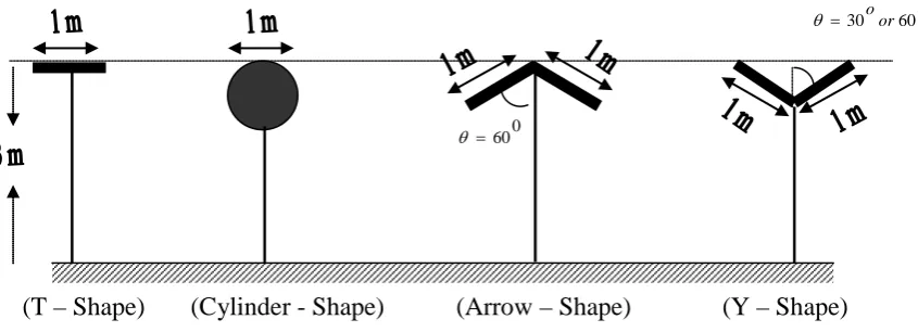
The performance of a few different shapes of single noise barriers with different upper edge

conditions has been predicted using 2D-boundary element method. The designs used in the

simulations are shown in Fig. 2.

The overall height of all type of barriers is fixed at 3 m, which is the same as that used in

the T top in T–shape barrier is 1 m, diameter in Cylinder is 1 m and the width of each side of

the caps in both Arrow and Y-shape is 1m. The angle of the arrow shape barrier is 60 degrees

while the angles for “Y” shape barrier are 30 and 60 degrees.

The above dimensions are similar to those used in previous studies [1,2,4]. Three different

surfaces were used on the barrier including rigid, absorbing and QRD coverage.

I. Rigid surface: All surface admittances are zero, which is the Neumann boundary condition.

II. Absorbing surface: Only the upper surface of the cap is covered with fibrous absorptive

material. A typical flow resistivity of 20000 Ns/m4 is assumed for the fibrous material. The

thickness of the fibrous material is fixed at 0.2445 m (the same as the thickness of the

QRD, see below). Barrier models with this absorptive cover are labelled with a prefix “A”

in this paper. For example a T-shape barrier with the absorptive cover is labelled as

AT-shape barrier.

III. QRD barrier: Quadratic residue diffusers with different designs are fixed to the upper

surface of barriers shown in Fig. 2 with the overall height remained constant. Different

designs are used to examine how diffusers affect the performance of barriers. The different

designs and their model names are given in Table 1.

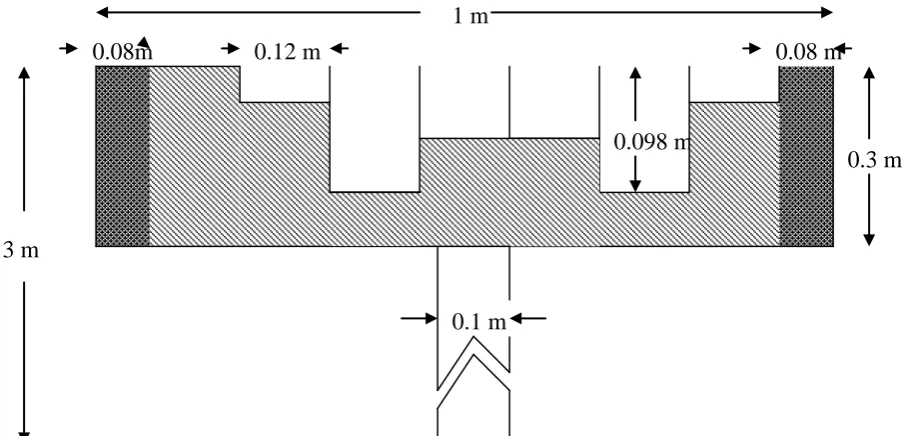
The dimension of one of the tested QRD designs (labelled model “A” here) is shown in detail

in Fig. 3. All other models are fitted in the same overall frame, so that the overall lengths of

all the QRD configurations used in different barrier models are the same. The maximum well

depth among all the QRD models, which corresponds to a QRD tuned at 400 Hz, is 0.2445 m.

This maximum depth was the same as the absorbent material thickness used in the last

section.

In order to investigate to what extent the QRD barriers improve the performance of different

forms of barriers, the results are compared against a reference barrier, which is chosen to be

the T shape barrier with the fibrous absorptive cover (labelled as AT shape barrier). For

convenience this model will also be referred as the “Ref” model.

) 2 ( ) mod ( 2 r n f N N n c

d = (4)

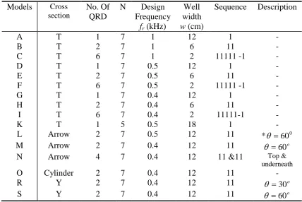
where n is an integer, N is an odd prime number and fr is the design frequency. Table 1 shows

the configurations of the different QRD barrier models. In this table under the column

“Sequence”, the sign “1” is for a sequence of 0 1 4 2 2 4 1 and the sign of “-1” is for an

inverse sequence.

The lower and upper wavelength limits can also be approximated roughly by [10]:

w n Nd 2 ; 2 min max max

max ≈ λ ≈

λ (5)

where dmax is the maximum depth and nmax is the maximum number from the sequence

(n2mod N). Therefore the frequency bandwidth for a N=7 QRD with well width of 12cm is

from fr to about 1.4 kHz, e.g. for a N=7 QRD with maximum depth of 0.2445m and a well

width of 12cm the frequency bandwidth should be from 400 to 1.4kHz. In practice the

frequency bandwidth is slightly wider than this.

In all calculations in this paper the fin thickness is assumed to be negligible. If the surfaces of

the wells are rigid and it is sufficiently wide for viscous and thermal condition to be

negligible then the specific input admittance at the open side of the channel can be

represented approximately as:

) tan(kd j − = β (6)

where k is the wave number and d is the well depth.

a. Whole surface modelling

As it was mentioned earlier in this paper the main BEM calculation is based on the

assumption that the QRD can be represented by box with a variable impedance surface. The

accuracy of this assumption is determined by comparing a prediction using this assumption

with a prediction that model the exact geometry of the QRD, which is referred to as “whole

surface modelling” here. The comparison is made on the most frequent used barrier in this

study, model “G”, in Fig. 4. In this model the fin thickness is 5 mm. Apart from the fins,

the size of elements remains the same as in the box approximation method. As expected,

1.4kHz in this case. Above the upper cut off frequency, i.e. above the design frequency

range of the QRD, the overall trends of the 2 predictions are still similar but the box

approximation gives rise to noticeable error, which can be about 5dB at certain single

frequencies. With this in mind, the box approximation is a convenient and accurate

representation for the investigation of QRD barrier performance within and under the

design frequency range of the QRD.

b. QRD edged barriers of different shapes

In order to give a clear demonstration of the results for different basic barrier shapes, the four

models, G, O, M and R are compared with their original rigid and absorbent shapes. These

four models have the same QRD design, with the same frequency design, which is 400 Hz,

and the same well width of 12cm. In other words the QRDs used in these models have the

same frequency bandwidth (from about 400Hz to 1.4kHz), and the only difference is the

shape of the barrier top that the QRDs are fitted into.

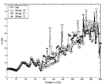
Employing the designed QRD on model “G” (T-shape) increases significantly the insertion

loss of the barrier compared with both rigid and absorbent T-shape profiles at frequencies

above 315 Hz. Fig. 5.a clearly shows the peaks of insertion loss gained by model “G” at

315,630 and 1000 Hz. Increases at 400 Hz, 1.25 kHz and 2 kHz are also significant. At

frequencies lower than 315 Hz and above 2 kHz (outside the QRD frequency bandwidth) the

performance start to decline and go even slightly lower than rigid shape at very low

frequencies. It is worth noting that only one QRD period is used in this model.

In Fig. 5.b two identical QRD periods (fr=400 Hz, w =0.12 m) are used on the cylinder

profile. In this model the first significant peak is at 315 Hz, the second and third visible peak

630 Hz and 1.25 kHz respectively.

Utilising two identical QRDs (fr=400 Hz, w=0.12 m) on an Arrow-shape barrier significantly

improves the performance compared with the corresponding rigid and even the absorptive

arrow shape barriers as one can see in Fig. 5.c. There are successive peaks in the frequency

spectrum that push the performance of the model “M” barrier significantly higher than the

315 Hz. The peaks at 1 kHz and 1.25 kHz are also significant. As expected at frequencies

higher than 1.6 kHz (above the upper cut-off frequency of the QRD) the QRD barrier

becomes less efficient, but the absorbent barrier is still significantly better than that of rigid

shape barrier.

On the Y-shape barrier employing two identical QRDs doesn’t show significant

improvements. As it is shown in Fig. 5.d, although two peaks at 250 Hz and 1 kHz are higher

than the absorbent Y- shape the trends of all three Y-shape models are very close to each

other in the entire frequency spectrum. This is because the QRDs and likewise the absorptive

surfaces are not facing the source and receiver.

A common effect of the QRDs on all the different barrier models is that the barrier IL

becomes more frequency dependent compared with the rigid and absorbent equivalents.

There are significant peaks occurring in the frequency spectrum. This is consistent with the

operational characteristics of a QRD in which well resonances occur at various frequencies

corresponding to the well depth sequence. The best improvement is seen within the design

frequency bandwidth of the QRD from about 315Hz to 1.4kHz, with also noticeable

improvements at 2 kHz in model “G” and at 250 Hz in model “S”. Every models show a

significant peak at 1 kHz. In all cases the employment of QRD improves the performance of

the barriers within the design frequency bandwidth of the QRD.

c. Barrier configurations with different QRD designs

The calculated spectra of insertion loss of all tested models with a T- shape profile are shown

in Fig. 6. For clarity the results are split to four graphs. Fig. 6.a, b, and c have QRDs with

prime number 7, and show performance variations due to frequency design and different well

width. Within each subplot the design frequency is the same but the well width is reduced

from 12cm to 6cm and then 2cm. This results in higher upper cut-off frequencies and larger

numbers of QRD periods for the smaller well widths. The design frequencies are 1kHz,

500Hz and 400Hz respectively for the QRDs in Figures 6.a, 6.b and 6.c. The effect of

reducing the prime number is shown in Fig. 6.d, in which model “K” has a QRD with N=5

There are common trends in Fig. 6.a, b and c, which are related to the design frequency and

the well width of the QRD. It is clear that lowering the design frequency of the QRD shifts

the first peak of the insertion loss of the QRD barrier to a lower frequency. Indeed the

frequency of the first peak is very close to the design frequency, again evidence that the

peaks in the insertion loss are strongly related to the characteristic resonances of the QRD

wells. The effect of decreasing the well width is not as clear. In theory a smaller well width

gives a higher upper cut-off frequency to the QRD and therefore should result in better

performance at higher frequencies. This is not shown by this simulation. This is a limitation

of the current assumption used in the numerical modelling in which the QRD is approximated

by a box with surface admittance distribution given by the simple plane wave admittance of

the QRD wells. This approximation is maintained even at frequencies above the QRD’s upper

cut-off frequency above which the plane wave assumption is no longer adequate. Hence

results above the cut-off frequencies (1.4kHz for w=12cm, 2.8kHz for w=6cm, and 8.4kHz

for w=2cm) may not be accurate, as already been discussed earlier under Figure 4. Below the

upper cut-off, a decrease in well width sometime increases the performance of the barrier at

peak points, however the efficiency is decreased at the minimum points with the overall

effect that the broadband mean insertion loss remained roughly unchanged. It should be

reminded that viscous and thermal loses were ignored in the calculation of the QRD

admittance. For very small well widths, these effects could be significant and introduce larger

impedance as well as significant absorption [11, 12].

In Figure 6.d, the reduction in the QRD prime number changes the maximum and minimum

frequencies over which the QRD is effective. The frequency at which the barrier with QRD

with N=5 starts to become effective is 250 Hz and the second and the third peaks appears at 1

kHz and 1.6 kHz. More importantly, Fig 6.d clearly shows that a QRD with a smaller prime

number N has less peaks in the insertion loss spectrum. With a smaller N the number of

different well depths is reduced. As a consequence the number of well resonances, and hence

the insertion loss peaks, is also reduced. In Figure 6.d, although the increases in insertion loss

at the peaks at 315Hz , 1kHz and 1.6 kHz are significant, the insertion loss in between is no

more than that provided by the equivalent rigid T-shape barrier. The result strongly suggests

that a QRD with a larger variation of well depths (larger N) will perform better when applied

Using two QRDs on two different configurations of Y-shape barrier with, 30 and 60 degrees

of the Y-angle, made the two barrier models “R” and “S”. Their performances are compared

with the T- shape barrier in Fig. 7. Increase the angle from 30 to 60 degrees could raise the

gained insertion loss between 200 Hz and 3.15 kHz, although at frequencies bellow 200 Hz

the situation is the opposite. Overall the 60 degrees Y-shape barrier performs better with the

QRD than the 30 degrees barrier, which is not surprising since a larger Y-angle exposes

larger portion of the QRD surface to the source and receiver.

d. QRD barrier top compared with absorptive top

According to Hothersall et al. [1] T-shape profile barriers with strongly absorbent materials

on the top surface of the T- part was the best choice among barrier design he investigated.

Fig. 8 and 9 compare the new QRD barrier designs in this research with the equivalent

absorbent T-shape barrier, labelled “Ref” in the figures. In all cases the barriers have the

same overall height, thickness, source, receiver and ground conditions. Significant

improvement is provided by model “G” (T- shape profile with one period of the N=7,

fr=400Hz QRD) at frequencies above 315 Hz as shown in Fig. 8. The other two QRD models

also improve the efficiency of the barrier but at higher starting frequencies because of their

higher design frequencies.

The A- weighted road traffic noise spectrum [13] is calculated by combining the results for

insertion loss at one-third octave band centre frequencies over the range 50 to 4000 Hz and

assuming a suitable source spectrum. It is usually done to average the interference effects

observed at single frequencies, and allow smoother trends to be identified more easily. It is

worth adding that the result in 1/15 octave band was averaged to give 1/3-octave band based

on simple energy averaging method. At receiver point (50,0) the A- weighted road traffic

noise is 14.5, 15.8 and 15.9 dB(A) for model “A”, “D” and “G” respectively, compared with

15.7 dB(A) for the “Ref” barrier. Model “G” enhances the mean insertion loss by a further

0.2 dB(A) compared with an absorbent T- shape barrier at this receiver point.

The effect of the QRD on an Arrow shape barrier (model “M”) is also compared with the

reference absorbent T shape barrier in Fig. 9. The influence of the QRD on an Arrow shape

barrier (model “M”) is stronger than on a T-shape barrier (model “G”) in the frequency range

e. IL difference of QRD top barriers with Reference barrier

A calculation has been carried out to find the increase in the barrier insertion loss, ∆IL,due to

the application of the QRD to show the domain of improvement of selected models compare

to the absorbent T- shape “Ref” barrier. In each frequency the insertion loss of the selected

model is subtracted by that of the “Ref” model. Fig. 10 and 11 show the results.

While the effect of model “G” (T-shape) is mainly between 315 Hz to 1.25 kHz, the effective

frequency domain of model “M” (Arrow-shape) is extended one 1/3 octave band below and

above that of model “G”. Outside the effective frequency domain the insertion loss in model

“G” is about the same as that of an equivalent absorbent T-shape barrier. However the

reduction at frequencies below 250 Hz is rather significant in model “M”.

Fig.11 shows a clear view of the effect of different frequency designs of QRD on the barrier

models compared to the “Ref” absorbent T- shape barrier. All three QRD models improve the

efficiency of the barrier significantly within their respective frequency bandwidths. Decrease

in the design frequency shifts the effective frequency domain towards lower frequencies. So

the first effective frequency for model “A” (fr=1 kHz) is 630 Hz while that for model “D” (fr

=500 Hz) is 315 Hz and finally 250 Hz is the starting effective frequency for model “G” (fr

=400 Hz).

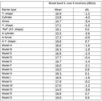
f. Broad band insertion loss

The broadband insertion loss at nine receiver positions 20, 50 and 100 m from the centre line

of the barrier on the ground and at 1.5 and 3 m above the rigid ground for the A-weighted

traffic noise spectrum [13] are shown in Table 2. The insertion loss over the receiver positions for each barrier and the ΔIL, which is the difference in the mean insertion loss relative to the reference absorbent T-shape barrier are also shown. Using QRD on the Arrow-

shape and cylindrical shape barrier (model “O”) could not improve the A- weighted mean

insertion loss of the barriers compare to the reference barrier. Different forms of the Y-shape

barrier, either absorbent or QRD tops (models “R” and “S”), have slightly higher mean

It is worth noting that employing a QRD with fr=400 Hz on both T-shape and Y- shape raises

the mean insertion loss of all barrier shapes (except Model “I”) beyond that of the “Ref”

absorbent T-shape barrier. Using this QRD tuned to 400 Hz on a rigid T-shape barrier (model

“G”) improves the efficiency of the barrier by 0.9 dB(A) compared with that of the reference

absorbent T-shape barrier.

Reducing the frequency design of the QRDs from 1 kHz (model “A”) to 500 HZ (model “D”)

and even lower down to 400 Hz (model “G”) improved the A- weighted insertion loss of

barriers from 16.6 dB (A) in model “A” to 17.7 dB (A) in model “D” and 19 dB(A) in model

“G”, which could be explained by the shifting of the frequency effect to low frequencies by

QRDs with lower frequency design.

Although reducing the well width of the applied QRDs could potentially increase the

absorption coefficient of the device [12], it is shown that it has negative effect on the A-

weighted insertion loss of any T – shape QRD barriers with different frequency designs

(except model “C” with a slight improvement). In this case reducing the well width in a

QRD tuned to 400 Hz from 12 cm in model “G” to 2 cm in model “I” decreased the

A-weighted insertion loss of the barriers from 19 dB(A) to 16.6 dB(A) respectively.

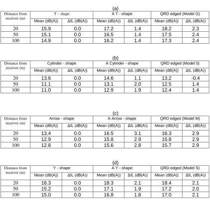
In fact in all types of barriers investigated both absorbent material and QRD (apart from

model “O” at 20 m distance from barrier) can improve the efficiency of the barrier compare

to their corresponding rigid shapes on the ground, as shown in Table 3. However the amount

of increase is dependent on the profile of the barriers. For example while covering the top

surface of Arrow-shape barrier with QRD improves the mean insertion loss by 2.9 dB(A) at

all receiver positions, the improvement for a Y-shape barrier is only about 2 dB(A). In T-

shape barrier the improvement provided by the QRD is higher than that provided by the

absorbent material. It should also be noted that the QRDs used in the investigation are

non-absorptive. It will be an interesting further work to investigate if an absorptive QRD, as

suggested in References [11, 12], can further improve the performance of a QRD barrier.

Furthermore as one can also see from Table.3 that the T- shape profile, with improvement

between 0.9 to 1 dB(A) due to QRD compare to its equivalent absorptive configurations, is

the best form to use QRD on. In contrast the Cylinder - shape profile, with between 0.5 to 1.4

g. Sound field at the shadow zone

The details of the far and near field effect of the presented models are shown in Figures 12 to

13 in contour plots of the broadband differences of A-weighted insertion loss relative to the

“Ref” absorptive T-shape barrier and absorbent Arrow - shape at 400 receiver positions for

two selected models: QRD barrier model “G” and “M”. Fig. 12 shows that model “G” (QRD

on T-shape) has got better performance in two distinctive areas of very close to the ground

and the field beyond 10 m from the barrier where the mean insertion loss increase is notably

higher at longer distances with higher height. The amount of improvement in the far field at

the height of 6 to 8 m can reach up to 2.5 to 3.5 dB(A), while the same amount of

improvement is visible at zones close to the ground in both near and far field. Close to the

barrier, especially at high receiver heights, the improvement is small to negative. This is

probably due to more sound being diffracted upwards by the QRD, which also explains the

higher insertion loss in the far field receiver and lower heights.

Fig. 13 shows that the performance of model “M” (QRD on Arrow-shape) is higher than its

equivalent absorbent Arrow – shape in the far filed at the height above 3 m. It produces 1.5 to

2 dB (A) higher insertion loss than the absorbent Arrow-shape barrier in the far field and

height of 6 to 8 m, similar to what is seen for model “G” in Fig. 12. Unlike model “G” the

improvement made by QRD on Arrow shape profile is very small to negative close to ground.

The area of negative effect is widened at the far field.

5.

Discussion and conclusion

The attenuation of sound by QRD edged single noise barriers has been investigated using a

two-dimensional boundary element model. Broadband insertion loss has been predicted over

a range of representative receiver positions using a A-weighted traffic noise spectrum in

1/15-octave band from 50 Hz to 4000 Hz. The performance of three different top surfaces;

rigid; absorptive; and QRD on four different types of barriers; T-shape; Cylindrical;

Arrow-shape; and Y-shape has been evaluated. The performances of QRD barriers have been

reference absorbent T- shape profile (the “Ref” model). The results can be summarised as

follows:

i. As already described in previous works, utilising absorbent material on the top

surface of a barrier could improve the efficiency of barriers. The best profile for using

absorption was found here to be the Arrow-shape with a 2.9 dB(A) mean insertion

loss improvement on the ground 50 m far from barrier. This was explained by the

high proportion of the treated surfaces facing the source and receiver in this barrier

profile

ii. Every single QRD barrier could increase the performance of rigid barrier within

certain frequency domain depending on its frequency design. It is possible to shift the

frequency effect to higher or lower frequencies by changing the utilized QRD

frequency design.

iii. Utilising QRD on different barrier profiles was found to produce insertion loss that

varies significantly with frequency and is strongly dependent on the design frequency

of the QRD. Overall, the numerical simulations in this study have shown that using

QRD to cover the top surface of T- shape and Y- shape barrier produces higher barrier

A-weighted insertion loss than using a typical fibrous absorbent material on the

barrier.

iv. Among the three different design frequencies tested, namely 1000, 500 and 400 Hz,

the most efficient design was found to be a QRD tuned to 400 Hz. As expected,

lowering the design frequency while keeping the upper cut-off frequency constant

provided higher broadband mean insertion loss.

v. It is found that putting one QRD with a design frequency of 400Hz on each side of an

Arrow-shape barrier could improve the mean broadband insertion loss of the barrier at

nine different receiver positions above the ground by 2.3 dB(A) . The amount of

improvement in mean insertion loss with a 400 Hz tuned QRD T-shape barrier

compare to an equivalent absorbent T-shape barrier was found to be 0.9 dB(A). In

contrast, using QRDs on cylindrical top barrier was found to decrease the A-weighted

performance of the absorbent profile barrier by 1 dB(A) .

vi. Reducing the well width of utilised QRD on T- shape profile barriers reduces the

vii. Employing QRD with less prime number resulted in fewer frequency peaks in the

insertion loss spectrum, although the overall barrier performance is slightly higher

than model “D” with the same frequency design but smaller well width.

viii. The QRD covered T-shape barrier (model “G”) was found to be effective in both the

far field at distance larger than 10 m from the barrier and areas close to the ground.

The efficiency of model ”G” is less than its equivalent absorbent barrier at the areas

close to the barrier above 3 m height. For the Arrow - shape QRD design the insertion

loss at areas close to the ground could be less than that of its equivalent absorptive

barrier.

It should be noted that the above results were obtained purely by numerical simulations.

Although the boundary element method used for the simulation has been found in previous

studies to have very good accuracy when applied to rigid and absorptive, and reactive

profiled barriers [1,2,4] and to QRD at normal incidence [10], its accuracy when dealing with

QRD on a barrier has yet to be confirmed with measurements. Furthermore the numerical

models assume that the admittance distribution on the QRD top surface is given by the simple

plane wave admittance of the well sequence. This assumption will break down at frequencies

above the upper cut-off frequency of the QRD as shown in Fig. 4. The viscous and thermal

losses in the wells will also complicate the admittance especially when the well width is

small. Besides, environmental factors such as atmospheric turbulence may further limit the

increase in insertion loss that could be obtained by the application of the QRD. Further work

Table 1. Design model names and corresponding configurations.

Models Cross section

No. Of QRD

N Design Frequency

fr (kHz)

Well width w (cm)

Sequence Description

A T 1 7 1 12 1 -

B T 2 7 1 6 11 -

C T 6 7 1 2 11111 -1 -

D T 1 7 0.5 12 1 -

E T 2 7 0.5 6 11 -

F T 6 7 0.5 2 11111 -1 -

G T 1 7 0.4 12 1 -

H T 2 7 0.4 6 11 -

I T 6 7 0.4 2 11111-1 -

K T 1 5 0.5 18 1 -

L Arrow 2 7 0.5 12 11 _* 0

60

= θ

M Arrow 2 7 0.4 12 11 o

60

= θ

N Arrow 4 7 0.4 12 11 &11 Top &

underneath

O Cylinder 2 7 0.4 12 11 -

R Y 2 7 0.4 12 11 o

30

= θ

S Y 2 7 0.4 12 11 o

60

= θ

Table 2. Broadband A-weighted mean insertion loss at nine receivers for various forms of

barriers. A typical traffic loss spectrum is assumed.

Broad band IL over 9 receivers (dB(A)) Barrier type Mean ΔIL

T- shape 16.9 -1.2

Cylinder 13.8 -4.3

Arrow 14.7 -3.4

Y- shape 17.1 -1.0

“Ref” (AT- shape) 18.1 0.0

A cylinder 15.5 -2.6

A Arrow _{17.2 -0.9}

A Y- shape 18.8 0.7

Model A 16.6 -1.6

Model B 16.3 -1.8

Model C 16.8 -1.3

Model D 17.7 -0.4

Model E 16.7 -1.4

Model F 16.0 -2.1

Model G _{19.0 0.9}

Model H _{18.3 0.1}

Model I 16.6 -1.6

Model K 17.9 -0.2

Model M 17.0 -1.2

Model O 14.5 -3.6

Model R 18.8 0.7

Model S _{19.0 0.9}

Table. 3. A comparison of broadband A- weighted mean insertion loss at three different receiver points on the ground for each barrier type having different top coverings: rigid, absorptive and QRD. (a) T- shape, (b) Cylinder- shape (c) Arrow- shape, (d) Y- shape.

(a) Distance from

receiver (m)

T – shape A T - shape QRD edged (Model G) Mean (dB(A)) ΔIL (dB(A)) Mean (dB(A)) ΔIL (dB(A)) Mean (dB(A)) ΔIL (dB(A))

20 15.9 0.0 17.2 1.4 18.2 2.3

50 15.1 0.0 16.5 1.4 17.5 2.4

100 14.9 0.0 16.2 1.4 17.3 2.4

(b) Distance from

receiver (m)

Cylinder - shape A Cylinder - shape QRD edged (Model 0) Mean (dB(A)) ΔIL (dB(A)) Mean (dB(A)) ΔIL (dB(A)) Mean (dB(A)) ΔIL (dB(A))

20 13.6 0.0 14.6 1.1 13.2 -0.4

50 11.1 0.0 13.1 2.0 12.5 1.4

100 11.0 0.0 12.9 1.9 12.4 1.4

(c) Distance from

receiver (m)

Arrow - shape A Arrow - shape QRD edged (Model M) Mean (dB(A)) ΔIL (dB(A)) Mean (dB(A)) ΔIL (dB(A)) Mean (dB(A)) ΔIL (dB(A))

20 13.4 0.0 16.5 3.1 16.3 2.9

50 12.9 0.0 15.8 2.9 15.8 2.9

100 12.8 0.0 15.6 2.8 15.7 2.9

(d) Distance from

receiver (m)

Y - shape A Y - shape QRD edged (Model S) Mean (dB(A)) ΔIL (dB(A)) Mean (dB(A)) ΔIL (dB(A)) Mean (dB(A)) ΔIL (dB(A))

20 16.3 0.0 18.3 2.1 18.4 2.1

50 15.2 0.0 17.1 1.9 17.2 2.0

100 15.0 0.0 16.8 1.8 17.0 2.1

References

1. D.C. Hothersall, D.H. Crombie, and S.N. Chandler-Wilde, “The performance of T-shape profile and associated noise barriers”, Applied Acoustics 32(4), pp.269-281, 1991.

2. D.H. Crombie, D.C. Hothersall, and S.N. Chandler-Wild, “Multiple-edge noise barrier”, Applied Acoustics 44(4), pp.353-367, 1995.

3. P. Menounou, I.J. Busch-Vishniac, D. T. Blackstock, “Directive line source model: A new model for sound diffraction by half planes and wedges”, J. Acoust. Soc. Am. 107 (6), pp.2973-2986, 2000.

4. Kyoji Fujiwara, David C. Hothersall and Chul-hwan Kim, “Noise barriers with reactive surfaces”, Applied Acoustics, 53 (4), pp. 225-272, 1998.

5. R. Seznec, “Diffraction of sound around barriers: use of boundary elements technique”, Journal of Sound Vibration 73(2), pp.195-209, 1980

6. D. C. Hothersall, S. N. Chandler-Wilde and M. N. Hajmirzae, “Efficiency of single noise barriers”, Journal of Sound Vibration, 146(2), pp.303-322, 1991.

7. M. E. Delany and E. N. Bazely, “Acoustical properties of fibrous absorbent material”, Applied Acoustics 3(2), pp.105-116, 1970.

8. Y. W. Lam and S. C. Roberts, “A simple method for accurate prediction of finite barrier insertion loss”, J.Acous.Soc.Am. 93, 1445-1452, 1993.

9. H. Kuttruff, “Sound absorption by psedostochastic diffusers (Schroeder diffusers)”, Applied Acoustics 42(3), pp.215-231, 1994.

10.Trevor J. Cox and Y. W. Lam, “Prediction and evaluation of the scattering from quadratic residue diffusers”, J. Acoust. Soc. Am. 95 (1), pp.297-305, 1994.

11.K. Fujiwara and T. Miyajima, “Absorption characristics of practically constructed Schroeder diffuser of quadratic-residue type”, Applied Acoustics 35(2), pp.149-152, 1992.

12.T. Wu, T. J. Cox, and Y. W. Lam, “From a profiled diffuser to an optimised absorber”, J. Acoust. Soc. Am . 108 (2), pp.643-650, 2000.

Figure Captions:

Figure 1. The two dimensional model.

Figure 2. Cross-sections of Barriers with Different Top Profiles.

Figure 3. Dimensions of the T- shape barrier having a QRD (N=7 and fr = 1 kHz).

Figure 4. Comparison between two prediction methods for model “G” at receiver point (-50,0).

Figure 5. Results of employing QRD tuned to 400 Hz on different barrier profiles at the receiver point (-50,0): with (a) T-shape (b) Cylinder - shape (c) Arrow-shape (d) Y- shape. Source is at (5,0).

Figure 6. Predicted frequency spectra of barrier insertion loss for ten different QRD T-shape barriers at the receiver point (-50, 0), with top surfaces having: (a) 1,2 & 6 QRDs (N=7 & fr

=1 kHz), (b) 1,2 & 6 QRDs (N=7 & fr =500 kHz), (c) 1,2 & 6 QRDs (N=7 & fr =400 kHz)

and (d) a QRD (N=5 & fr = 1 kHz). Well widths of the QRD changes within each subplot

according to Table 1.

Figure 7. Predicted spectra of Insertion Loss for QRD Y- Shape barriers along with T- Shape barrier at receiver point (-50,0).

Figure 8. The effect of QRD covers with different frequency designs compared with an absorptive cover on a T- shape barrier at the receiver point (-50,0).

Figure 9. A comparison between T- shape QRD barrier (Model “G”) and an Arrow - shape QRD barrier (Model “M”) with the “Ref” model at the receiver point (-50,0). The QRDs used are of the same design in both QRD barriers.

Figure 10. Differences in Insertion Loss of two QRD barrier models with the same QRD but different top profiles relative to that of the “Ref” model barrier at the receiver point (-50,0).

Figure 11. Differences of Insertion Loss of three QRD barrier models with different frequency designs relative to that of the “Ref” model barrier at receiver point (-50,0).

Figure 12. Contour plot of differences of broad band A- weighted insertion loss of barrier model “G” relative to “Ref” at 400 receiver positions.

y Barrier

Source γ

* r0

x

Figure 2. Cross-sections of Barriers with Different Top Profiles.

o or o

60 30

= θ

0 60 =

θ

Figure 3. Dimensions of the T- shape barrier having a QRD (N=7 and fr = 1 kHz).

1 m

0.3 m 0.08 m 0.12 m

0.08m

0.098 m

Figure 6. Predicted frequency spectra of barrier insertion loss for ten different QRD T-shape barriers at the receiver point (-50, 0), with top surfaces having: (a) 1,2 & 6 QRDs (N=7 & fr =1 kHz), (b) 1,2

& 6 QRDs (N=7 & fr =500 kHz), (c) 1,2 & 6 QRDs (N=7 & fr =400 kHz) and (d) a QRD (N=5 & fr =

Figure 13. Contour plot of differences of broad band A- weighted insertion loss of barrier model “M” relative to its equivalent absorbent Arrow – shape barrier at 400 receiver