THE EFFECT OF PRE-PROCESSING TECHNIQUES AND OPTIMAL PARAMETERS ON BPNN FOR DATA CLASSIFICATION
AMEER SALEH HUSSEIN
A dissertation submitted in Partial
fulfillment of the requirement for the award of the Degree of Master of Computer Science (Soft Computing)
Faculty of Computer Science and Information Technology Universiti Tun Hussein Onn Malaysia
ABSTRACT
The architecture of artificial neural network (ANN) laid the foundation as a powerful technique in handling problems such as pattern recognition and data analysis. It’s data-driven, self-adaptive, and non-linear capabilities channel it for use in processing at high speed and ability to learn the solution to a problem from a set of examples. It has been adequately applied in areas such as medical, financial, economy, and engineering. Neural network training has been a dynamic area of research, with the Multi-Layer Perceptron (MLP) trained with back propagation (BP) mostly worked on by various researchers. However, this algorithm is prone to have difficulties such as local minimum which are caused by neuron saturation in the hidden layer. Most existing approaches modify the learning model in order to add a random factor to the model which can help to overcome the tendency to sink into local minima. However, the random perturbations of the search direction and various kinds of stochastic adjustment to the current set of weights are not effective in enabling a network to escape from local minimum within a reasonable number of iterations. In this research, a performance analysis based on different activation functions; gradient descent and gradient descent with momentum, for training the BP algorithm with pre-processing techniques was executed. The Min-Max, Z-Score, and Decimal Scaling Normalization pre-processing techniques were analyzed. Results generated from the simulations reveal that the pre-processing techniques greatly increased the ANN convergence with Z-Score producing the best performance on all datasets by reaching up to 97.99%, 95.41% and 96.36% accuracy.
vi
ABSTRAK
Reka bentuk rangkaian neural tiruan (ANN) menyediakan asas sebagai teknik yang berkesan dalam pengendalian masalah seperti pengecaman corak dan analisis data. Keupayaannya yang dipacu data, penyesuaian kendiri, dan bukan linear menjadikannya boleh digunakan dalam pemprosesan pada kelajuan yang tinggi dan keupayaan untuk mempelajari penyelesaian masalah daripada satu set contoh. Ia telah diaplikasikan dalam bidang seperti perubatan, kewangan, ekonomi, dan kejuruteraan. Latihan rangkaian neural menjadi satu bidang penyelidikan yang dinamik, dengan Perseptron Berbilang Lapisan (MLP) dilatih dengan rambatan balik (BP) yang kebanyakannya telah dijalankan oleh pelbagai penyelidik. Walau bagaimanapun, algoritma ini cenderung untuk mempunyai kesukaran seperti minimum setempat yang disebabkan oleh ketepuan neuron dalam lapisan tersembunyi. Kebanyakan pendekatan sedia ada mengubah suai model pembelajaran untuk menambah satu faktor rambang kepada model berkenaan yang boleh membantu bagi mengatasi kecenderungan untuk terdorong ke dalam minimum setempat. Walau bagaimanapun, pengusikan rawak terhadap arah carian dan pelbagai jenis pelarasan stokastik kepada set pemberat semasa tidak berkesan bagi membolehkan sesuatu rangkaian untuk menjauhi daripada minimum setempat dalam jumlah lelaran yang munasabah. Dalam kajian ini, analisis prestasi berdasarkan fungsi pengaktifan berbeza; turunan cerun dan turunan cerun dengan momentum, untuk latihan algoritma BP dengan teknik prapemprosesan telah dilaksanakan. Teknik-teknik prapemprosesan Min-Max, Skor-Z, dan Penormalan Skala Perpuluhan telah dianalisis. Hasil yang dijana daripada simulasi-simulasi tersebut menunjukkan bahawa teknik prapemprosesan banyak meningkatkan penumpuan ANN dengan Skor-Z menghasilkan prestasi yang terbaik pada semua set data yang menjangkau ketepatan sehingga 97.99%, 95.41% dan 96.36%.
TABLE OF CONTENTS
DECLARATION ii
DEDICATION iii
ACKNOWLEDGEMENT iv
ABSTRACT v
ABSTRAK vi
TABLE OF CONTENTS vii
LIST OF TABLES x
LIST OF FIGURES xi
LIST OF SYMBOLS AND ABBREVIATIONS xiii
LIST OF APPENDICES xv
CHAPTER 1 INTRODUCTION 1
1.1 Overview 1
1.2 Problem Statement 2
1.3 Aim of the Study 4
1.4 Research Objectives 4
1.5 Scope of Study Research 4
1.6 Significance of the Study 5
1.7 Thesis Outline 5
CHAPTER 2 LITERATURE REVIEW 7
viii 2.2 Biological Neuron transformation to Artificial
Neuron (Perceptron) 8
2.3 Artificial Neural Network (ANN) 9
2.4 Component of Neural Network 10
2.4.1 Neuron 11 2.4.2 Weight 11 2.4.3 Hidden layer 12 2.4.4 Activation Function 12 2.4.4.1 Threshold Function 14
2.4.4.2 Piecewise Linear Function 14
2.4.4.3 Uni-Polar Sigmoidal Function 15
2.4.4.4 Hyperbolic Tangent Function 15
2.5 Multi-Layer Perceptron (MLP) 16 2.6 Back-Propagation Algorithm (BP) 17
2.7 Learning Algorithm for ANN 20
2.7.1 Gradient Descent Back-propagation (GD) 22 2.7.2 Gradient Descent with Momentum (GDM) 23 2.8 Data pre-processing 24
2.9 Classification Using ANN 26
2.10 Chapter Summary 28
CHAPTER 3 RESEARCH METHODOLOGY 29 3.1 Introduction 29
3.2 Data Selection 30
3.2.1 Iris Plants database 31
3.2.2 Balance Scale database 31
3.2.3 Car Evaluation database 32
3.3 Pre-processing Data 33
3.3.1 Min Max Normalization 34
3.3.2 Z-Score normalization 35
3.3.3 Normalization by decimal scaling 35
3.4 Data Partition 36
3.5 Network Models Topology 36
3.5.2 Number of Hidden Nodes 37 3.6 Training of the Network 38
3.6.1 Training Parameter Used 38
3.6.1.1 Learning Rate 39 3.6.1.2 Momentum 39 3.6.1.3 Activation Function 40
3.6.2 Stopping Criteria 40
3.7 Technique 40
3.8 Model Selection 42
3.9 Performance Evaluation 42
3.10 Chapter Summary 43
CHAPTER 4 SIMULATION RESULTS AND ANALYSIS 44
4.1 Introduction 44
4.2 Experimental Design 44
4.3 Experimental setup 45
4.4 Performance Comparison between Different
pre-processing techniques 45
4.5 Chapter Summary 54
CHAPTER 5 CONCLUSIONS AND FUTURE WORKS 55
5.1 Introduction 55
5.2 Research Contribution 55
5.2.1 Objective 1: The Construction and Training
Model of ANN 56 5.2.2 Objective 2: Classify Data after
Pre-processing by Using the trained ANN
Model 56
5.2.3 Objective 3: Evaluate the Performance of
the trained ANN 57
5.3 Recommendation and Future Works 57
REFERENCES 58
APPENDIX A 67
x
LIST OF TABLES
2.1 Advantages and Disadvantages of Gradient Descent Back-propagation 23
3.1 Content of Datasets 31
3.2 Attribute details for iris dataset 31 3.3 Attribute details for balance scale dataset 32 3.4 Attribute details for car evaluation dataset 32 3.5 Class details for car evaluation dataset 33 3.6 Number of Input and Output Nodes for Each
Dataset 37
3.7 The Value of Parameters for GD and GDM
Training Algorithm 39
4.1 Number of Instances in Training and Testing
Data Set 45
4.2 Performance of the Accuracy of Different pre-processing techniques on All Dataset for Training Algorithms (GD and GDM) 47 4.3 Performance of the MSE of Different
pre-processing techniques on All Dataset for Training Algorithms (GD and GDM) 49 4.4 Performance of the CPU time of Different
pre-processing techniques on All Dataset for Training Algorithms (GD and GDM) 51 4.5 Performance of the Epochs of Different
pre-processing on All Dataset for Training
LIST OF FIGURES
2.1 Biological and Artificial Neuron 9
2.2 Activation function 12
2.3 Types of Activation Function 16
2.4 Fully connection feed-forward network with one hidden layer and one output layer 17
2.5 Back-propagation Neural Network 19
2.6 Tasks in data pre-processing 25
3.1 Research methodology 30
4.1 The Accuracy of Different pre-processing techniques All Dataset for Training
Algorithm (GD) 47
4.2 The Accuracy of Different pre-processing techniques on All Dataset for Training
Algorithm (GDM) 48
4.3 The MSE of Different pre-processing techniques on All Dataset for Training Algorithm (GD) 49 4.4 The MSE of Different pre-processing techniques
on All Dataset for Training Algorithm (GDM) 50 4.5 The CPU Time of Different pre-processing
techniques on All Dataset for Training
Algorithm (GD) 51
4.6 The CPU Time of Different pre-processing techniques on All Dataset for Training
Algorithm (GDM) 52
4.7 The Epochs of Different pre-processing techniques on All Dataset for Training
xii 4.8 The Epochs of Different pre-processing
techniques on All Dataset for Training
LIST OF SYMBOLS AND ABBREVIATIONS
AI - Artificial Intelligence
ANN - Artificial Neural Networks
BP - Back Propagation
MLP - Multi Layer Perceptron
Min-Max - Pre-processing Min-Max Normalization Decimal Scaling - Pre-processing Decimal Scaling Normalization Z-Score - Pre-processing Z-Score Normalization
Min-Max-Tansig - Min Max Normalization with sigmoid activation function
Min-Max –Logsig - Min Max Normalization with sigmoid activation function
Decimal Scaling- - Decimal Scaling Normalization with tangent Tansig activation function
Decimal Scaling- - Decimal Scaling Normalization with sigmoid
Logsig activation function
Z-Score-Tansig - Z-Score Normalization with tangent activation function
Z-Score-Logsig - Z-Score Normalization with sigmoid activation Function
BPNN - Back-Propagation Neural Network
GD - Gradient Descent
GDM - Gradient Descent with Momentum
FFNN - Feed Forward Neural Network
ACC - Classification Accuracy
MSE - Mean Squared Error
CPU - Central Processing Unit
xiv IEEE - Institute of Electrical and Electronics Engineering UTHM - University Tun Hussein Onn Malaysia
η - Learning Rate
α - Momentum
Tanh - Hyperbolic Tangent Function
w - The weight vector
f(.) - Activation function
hi - Hidden node
xi - Inputs
t - The expected value
δ - Error term
∆wij - The delta/gradient of weights
maxp - The maximum value of attribute
minp - The minimum value of attribute
mean (p) - Mean of attribute P
std (p) - Standard deviation of attribute P
m - Smallest integer number
A - The total number of instance
C - The corrected class
N - The number of instance
Pi - Vector of (n) predictions
Pi* - Vector of the true values
LIST OF APPENDICES
APPENDIX TITLE PAGE
A Figure A.I.1: The effect of learning rate on the Classification Accuracy using pre-processing techniques and training algorithm (GD) on Iris
data. 67
Figure A.I.2: The effect of learning rate on the MSE using pre-processing techniques and training algorithm (GD) on Iris data. 67 Figure A.I.3: The effect of learning rate value on CPU time using pre-processing techniques on training algorithm (GD) on Iris data. 68 Figure A.I.4: The effect of learning rate value on the Epochs using pre-processing techniques on training algorithm (GD) on Iris data. 68 Figure A.I.5: The effect of momentum on the
Classification Accuracy using pre-processing
techniques and training algorithm (GDM) on
Iris data. 69
xvi Figure A.I.8: The effect of momentum value on the Epochs using pre-processing techniques and training algorithm (GDM) on Iris data. 70 Figure A.II.1: The effect of learning rate on the Classification Accuracy using pre-processing
techniques and training algorithm (GD) on
Balance- Scale data. 71
Figure A.II.2: The effect of learning rate on the MSE using pre-processing techniques and training algorithm (GD) on Balance-Scale data. 71 Figure A.II.3: The effect of learning rate value on CPU time using pre-processing techniques and training algorithm (GD) on Balance-Scale
data. 72
Figure A.II.4: The effect of learning rate value on the Epochs using pre-processing techniques and training algorithm (GD) on Balance-Scale
data. 72
Figure A.II.5: The effect of momentum on the Classification Accuracy using pre-processing techniques and training algorithm (GDM) on
Balance-Scale data. 73
Figure A.II.6: The effect of momentum on the MSE using pre-processing techniques and
training algorithm (GDM) on Balance-Scale
data 73
Figure A.II.7: The effect of momentum value on CPU time using pre-processing techniques and training algorithm (GDM) on Balance-Scale
data. 74
Figure A.III.1: The effect of learning rate on the Classification Accuracy using pre-processing techniques and training algorithm (GD) on car
evaluation data. 75
Figure A.III.2: The effect of learning rate on the MSE using preprocessing techniques and training algorithm (GD) on car evaluation data. 75
Figure A.III.3: The effect of learning rate value on CPU time using pre-processing techniques and training algorithm (GD) on car evaluation
data. 76
Figure A.III.4: The effect of learning rate value on the Epochs using pre-processing techniques and training algorithm (GD) on car evaluation
data. 76
Figure A.III.5: The effect of momentum on the
Classification Accuracy using pre-processing techniques and training algorithm (GDM) on
car evaluation data. 77
Figure A.III.6: The effect of momentum on the MSE using preprocessing techniques and training algorithm (GDM) on car evaluation data. 77
Figure A.III.7: The effect of momentum value on CPU time using pre-processing techniques and training algorithm (GDM) on car
evaluation data. 78
Figure A.III.8: The effect of momentum value on the Epochs using pre-processing techniques and training algorithm (GDM) on car evaluation
1CHAPTER 1
INTRODUCTION
1.1 Overview
Artificial Neural Network (ANN) is an information processing paradigm motivated by biological nervous systems. The human learning process may be partially automated with ANNs, which can be constructed for a specific application such as pattern recognition or data classification, through a learning process (Mokhlessi & Rad, 2010). ANNs and their techniques have become increasingly important for modeling and optimization in many areas of science and engineering, and this assertion is largely attributed to their ability to exploit the tolerance for imprecision and uncertainty in real-world problems, coupled with their robustness and parallelism (Nicoletti, 1999). Artificial Neural Networks (ANNs) have been implemented for a variety of classification and learning tasks (Bhuiyan, 2009). As such, the reason for using ANNs rest solely on its several inhibitory properties such as the generalization and the capability of learning from training data, even where the rules are not known a-priori (Penedo et al., 1998).
certain threshold), the neuron is activated and emits a signal though the axon. This signal might be sent to another synapse and might activate other neurons.
The number of types of ANNs and their uses is very high. Since the first neural model by McCulloch and Pitts (1943), there have been hundreds of different models developed considered as ANNs. The differences in them might be the functions, the accepted values, the topology, the learning algorithms, etc. Also, there are many hybrid models where each neuron has more properties but focus is directed at an ANN which learns using the back-propagation algorithm (Psichogios & Ungar, 1992) for learning the appropriate weights. Furthermore, Back-Propagation (BP) is one of the most common models used in ANNs (Vogl et al., 1988).
Back-Propagation (BP), the most commonly used neural network learning technique, is one of the most effective algorithms accepted currently, and also the basis of pattern identification of BP neural network. Gradient based methods are one of the most commonly used error minimization methods used to train back-propagation networks. Despite its popularity, there exist some shortcomings such as the defects of local optimal and slow convergence speed, etc. (Tongli et al., 2013). There are many researches aimed at improving the traditional Back-Propagation Neural Network (BPNN) since 1986 such as the addition of learning rate, and momentum parameters, or use of different activation function etc. This research is trying to avoid some shortcomings in BPNN algorithm. The problem statement will be discussed in the next section.
1.2 Problem Statement
3 to add a random factor to the model, which can overcome the tendency to sink into local minima. However, the random perturbations of the search direction and various kinds of stochastic adjustments to the current set of weights are not effective in enabling a network to escape from local minima to converge to global minimum within a reasonable number of iterations (Vogl et al., 1988). There are many techniques used for improving training efficiency of back-propagation algorithm such as data pre-processing techniques that are considered the important steps in the data mining process. This research will investigate the following issues which affect the performance of BP algorithm:
i. Data is not properly pre-processed
Real-life data rarely complies with the requirements of various data mining tools. It is often inconsistent, noisy, contains redundant attributes and has unsuitable format, etc. That is why it has to be prepared carefully before the process of data mining can be started. It is well known that the success of every data mining algorithm strongly depends on the quality of data processing (Singh & Sane, 2014). In this context, it is natural that data pre-processing can be a very complicated task. Sometimes, data pre-processing takes more than half of the total time spent by solving the data mining problem. It is well known that data preparation is a key to the success of data mining tasks (Miksovskj et al., 2002). There are many techniques in pre-process data such as; Min-Max, Z-Score and Decimal Scaling Normalization preprocessing techniques. It is important to be able to identify which of the preprocessing methods will be adequately suitable in influencing and enhancing BP training.
ii. Some parameters that influence on the performance of BP
1.3 Aim of the Study
The aim of this study is to classify benchmarked data using Artificial Neural Networks technique by focusing on the effect of pre-processing techniques and different ANN algorithms.
1.4 Research Objectives
This research intends to do the following objectives;
i. To study the effects of some parameters in back propagation algorithm namely; learning rate η, momentum α, activation function with different pre-processing techniques namely; Min-Max, Z-Score and Decimal Scaling Normalization preprocessing techniques; in improving the classification accuracy on some classification problems.
ii. To apply a combination of data pre-processing technique with optimal parameters in BP training algorithm.
iii. To compare the performance of the combined techniques in (ii) with other (GD, GDM) traditional techniques in classifying some benchmarked problems.
1.5 Scope of Study
5 1.6 Significance of Study
The importance of this research is to increase the classification accuracy by using ANN model for classification problems. Classification technique is a complex and fuzzy cognitive process. Hence, soft computing methods such as artificial neural networks have shown great reliable potentials and power when applied to these problems. The use of technology especially ANN techniques in classifying application can reduce the cost time, human expertise and error. Therefore, the research significance will be focusing on improving BP training by integrating or combining the optimal data pre-processing technique with optimal parameters such as types of the activation function, learning rate, momentum term, number of hidden nodes in achieving good accuracy for classification problem on some benchmark dataset. The outline of the thesis will be discussed in the next section.
1.7 Thesis Outline
The thesis is subdivided into six chapters, including the introduction and conclusion chapters. The following is the synopsis of each chapter:
Chapter 1: Introduction. Apart from providing an outline of the thesis, this chapter contains an overview of the background to research work, research problem, objectives, research scope and methodologies in conducting this research.
introducing a proper technique for improving the learning efficiency as described in Chapter Three.
Chapter 3: Research Methodology. This chapter extends the work by using process technique as proposed in Chapter Two. It was discovered that the use of pre-process technique influences the BP performance. The descriptions of the steps on how to use the ANN models for classification of datasets are presented, starting from the variable and data selection, data pre-processing and data partition, and performance comparison of the different training algorithms and different activation functions. The rationale of selecting parameters for each algorithm, the evaluation covering all the network parameters: the hidden nodes higher order terms, the learning factors and momentum factor, also the number of output nodes in the output layer. The proposed workflow is programmed in MATLAB toolbox programming language and is tested for its correctness on selected benchmark data sets. The results of the proposed workflow were compared to facilitate further testing and validation in the next chapter.
Chapter 4: Results and Discussions. The simulation results of the pre-processing techniques with each training algorithm is discussed and presented in this section. The efficient workflow proposed in Chapter Three is further evaluated for its efficiency and accuracy on a variety of benchmark data sets. Each model is then presented graphically in the last chapter.
Chapter 5: Conclusion and future work. The research contributions are summarized
2CHAPTER 2
LITERATURE REVIEW
2.1 Introduction
Over five decades, during which Artificial Intelligence (AI) has been a defined and active field, in several literature surveys. However, the field is extraordinarily difficult to encapsulate either chronologically or thematically (Brunette et al., 2009). Artificial Neural Networks (ANNs) are a form of artificial computer intelligence which are the mathematical algorithms, generated by computers (Lei & Xing-Cheng, 2010). The Artificial Neural Networks (ANNs) has become popular recently and is one of the most effective computational intelligence techniques applied in Pattern Recognition Data Mining and Machine Learning (Nawi et al, 2013).
(Khemphila & Boonjing, 2010). Interestingly, the errors and undesirable results are reasons for a need for unconventional computer-based systems, which in turn reduces the errors, increases the reliability and safety (Ghwanmeh et al., 2013).
On the other hand, during the past few years, there have been significant researches on data mining particularly neural networks because it is heavily used in many fields. Most of these applications have used the back-propagation algorithm as the learning algorithm. The back-propagation algorithm requires the weights of each unit be adjusted so that the total quadratic error between the actual output and the desired output is reduced. A big problem with back-propagation networks is that its convergence time is usually very long. Selecting good parameters such as learning rate and momentum can reduce the training time but can require a lot of trial and error. Trying to find a universal learning rate or momentum which fits all needs is unrealistic (Hamid et al., 2011).
Therefore, this chapter focuses on the previous literature work that suggested certain improvements on BPNN model together with the effect of using pre-processing techniques for classification problems. The data mining processes and concepts constitute the section below.
2.2 Biological Neuron Transformation to Artificial Neuron (Perceptron)
The human brain which contains approximately 100 billion neurons - with 100 trillion connections, is an open complex giant system of self-organization and has two basic principles of organization: functional differentiation and functional integration (Huang & Feng, 2011).
9 information to each other. The link between two neurons is done via weighted connections (Lei & Xing-Cheng, 2010) and is depicted in Figure 2.1(b).
(a): Biological Neuron (Dohnal et al., 2005)
(b): Artificial Neuron (Dohnal et al., 2005)
Figure 2.1: Biological and Artificial Neuron
2.3 Artificial Neural Network (ANN)
The artificial neural networks are a branch of artificial intelligence and also a research domain of neuron informatics. They are made of simple processing units (artificial neurons) that are strongly interconnected and work in parallel. The artificial neurons are a conceptual model of biological neurons that are part of human nervous system. Therefore, these networks can be considered a simplified form of a human brain. Their aim is to interact with the environment the same way a biological brain would do this. They have some properties that bring them very close to this aim: the ability to perform distributed computations, to tolerate noisy inputs and to learn (Filimon & Albu, 2014).
and ability to process information. These results are stored within synaptic connections between neurons and existing network layers.
The main structure of the artificial neural network (ANN) is made up of the input layer, hidden layer, and the output layer (Li et al., 2014). Hence , Over the last few years, the artificial neural network (ANN) methodology has been accepted widely to solve problems such as prediction, classification, and ANN has become one of the most highly parameterized models that have attracted considerable attention in recent years (Isa et al., 2010). Because of the learning and self-organizing ability to adapt, artificial neural network (ANN) has the characteristics that can be trained. It can absorb experience by learning from the historical data and previous project information which can be used in the new prediction period. Back-propagation algorithm (BP) and feed-forward network are two widely applied ANN estimation technologies. ANN is constituted with active layers and hidden layers, and lots of nodes are connected inside each layer. One connection between two nodes represents a weight and each node represents a special activation function in which sigmoid function is widely used. ANN has the ability of self-learning process, modifying each layer’s weight by training samples. The widely used algorithm is Back-propagation (Dan, 2013).
2.4 Components of Neural Network
As the name suggests, an artificial neural network is a system that consists of a network of interconnected unit called artificial neurons. The units are called artificial neurons because of a certain resemblance to the neurons in the human brain (Dohnal et al., 2005). An ANN consists of an enormous number of massively interconnected
11 black box depends on the Neural Network structure and the model of every neuron in this structure.
2.4.1 Neuron
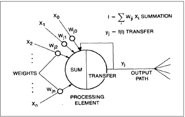
The artificial neuron model is a kind of artificial information processing model to extract, simplify, and imitate the creature neuron which is based on research for nerve science over the years (Lv et al., 2007). The artificial neuron is an information processing unit that is fundamental to the operation of a neural network, where it receives one or more inputs (representing the one or more dendrites) and sums them to produce an output (representing a biological neuron’s axon). Usually the sums of each node are weighted, and the sum is passed through a non-linear function known as an activation function or transfer function. The transfer functions usually have a sigmoid shape, but they may also take the form of other non-linear functions.
2.4.2 Weight
Neural networks often have a large number of parameters (weights) (Leung et al., 2003). Typically, a neuron has more than one input. A neuron with R inputs and the individual input ∑ 𝑥𝑅 are each weighted by corresponding elements ∑ 𝑤1𝑅 of the weight matrix W. A set of synapses or connecting links, each of which is characterized by a weight or strength of its own specifically a single (xj) at the input of synapses j connected to neuron K is multiplied by the synaptic weight (wkj). It is
important to make note of the manner in which the subscripts of the synaptic weight (wkj) are written, where the first subscripts refers to the neuron in question and the
2.4.3 Hidden layer
Multi-layer network consists of one or more layers of neurons called hidden layer between input and output layer (Svozil et al., 1997). Hence, the hidden layer units can be any number (normally decided from trial and error) and the accuracy of the approximation depends on the number of nodes in the hidden layers of multi-layered network. Meanwhile, number of hidden nodes equals half the sum of the number of input and output nodes (Nawi, 2014). Also, many researchers have used five hidden nodes and got good results with BP for different classification problems (Nawi et al., 2013; Isa et al., 2010; Hamid et al., 2011).
2.4.4 Activation Function
The activation function (also called a transfer function) shown in Figure 2.2, can be a linear or nonlinear function. There are different types of activation functions (Sibi et al., 2013). The activation function f(.) is also known as a squashing function. It keeps
[image:26.595.160.479.527.729.2]the cell’s output between certain limits as is the case in the biological neuron (Chandra & Singh, 2004). On the other hand, the relationship between the net inputs and the output is called the activation function of the Artificial Neuron. There could be different function or relationships that determine the value of output that would be produced for given net inputs.
13
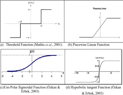
There are various types of activation functions such as; Threshold Function (hard-limiter), Piecewise Linear Function (Linear Function), Uni-Polar Sigmoidal Function (S-shape function) and Hyperbolic Tangent Function etc. Sigmoid and hyperbolic tangent are the most widely used because their differentiable nature makes them compatible with back propagation algorithm (BP). Both activation functions have an s-shaped curve while their output range varies.
The selection of activation function might significantly affect the performance of a training algorithm. Some researchers have investigated to find special activation function to simplify the network structure and to accelerate convergence time (Isa et al., 2010). Hence, in designing neural networks, fast learning with a high possibility of convergence and small network size are very important. They are highly dependent on network models, learning algorithms and problems to be solved. They are also highly related to activation functions (Nakayama & Ohsugi, 1998).
In Lee and Moraga (1996), a Cosine-Modulated Gaussian activation function for Hyper-Hill neural networks has been proposed. The study compared the Cosine-Modulated Gaussian, hyperbolic tangent, sigmoid and sym-sigmoid function in cascade correlation network to solve sonar benchmark problem. Joarder and Aziz (2002) proved that logarithmic function is able to accelerate back propagation learning or network convergence. The study has solved XOR problem, character recognition, machine learning database and encoder problem using MLP network with back propagation learning. Wong et al. (2002) investigated the neuronal function for network convergence and pruning performance. Periodic and monotonic activation functions were chosen for the analyses of multilayer feed forward neural networks trained by Extended Kalman Filter (EKF) algorithm. The study has solved multi-cluster classification and identification problem of XOR logic function, parity generation, handwritten digit recognition, piecewise linear function approximation and sunspot series prediction. Piekniewski and Tybicki (2004) employed different activation functions in MLP networks to determine the visual comparison performance.
2.4.4.1 Threshold Function
Threshold function for this type of activation function is depicted in Figure 2.3(a). Say there exists:
𝑔(𝑛𝑒𝑡) =�1: 0: 𝑖𝑓𝑖𝑓𝑛𝑒𝑡𝑛𝑒𝑡 ≥< 00 (2.1)
Correspondingly, the output of the neuron j employing such threshold function is expressed as:
𝑦𝑗 =�1: 𝑖𝑓 𝑛𝑒𝑡𝑗 ≥ 0
0: 𝑖𝑓 𝑛𝑒𝑡𝑗 < 0 (2.2)
where net j is the net input applied to neuron j; that translates to:
𝑛𝑒𝑡𝑗 = ∑𝑘𝑗=0 𝑤𝑗𝑘𝑥𝑘 (2.3)
Such a neuron is referred to in literature as the McCullocb-Pitts model which is in recognition of the pioneering work done by McCulloch and Pitts. In this model, the output of the neuron takes the value 1 if the total internal activity level at that neuron is nonnegative and 0 otherwise. This statement describes the all - or - none property of the McCullocb-Pitts model (Biol, 2011).
2.4.4.2Piecewise Linear Function
For Piecewise Linear Function depicted in Figure 2.3(b), there exists:
𝑔(𝑛𝑒𝑡) =
⎩ ⎪ ⎨ ⎪
⎧1: 𝑖𝑓𝑛𝑒𝑡 ≥12 𝑛𝑒𝑡: 𝑖𝑓 12> 𝑛𝑒𝑡 >−12 0: 𝑖𝑓𝑛𝑒𝑡 ≤ −12
(2.4)
15 The one extreme happens when the domain of the net input values for which this function is linear is infinite; then an activation function that is linear everywhere is being dealt with. The other extreme occurs when the domain of the net values for which activation function is linear shrinks to zero; in that case, threshold activation function comes into play (Sibi et al., 2013).
2.4.4.3 Uni-Polar Sigmoidal Function
Sigmoid function is by far the most common form of an activation function used in the construction of artificial neural networks (Xie, 2012). Activation function of Uni-polar sigmoid function is given as follows:
𝑔(𝑥) =1+𝑒1(−𝑥) (2.5)
This function is especially advantageous to use in neural networks trained by back-propagation algorithms. This is because it can be easily distinguished, and this can interestingly minimize the computation capacity for training. The term sigmoid means ‘S-shaped’, and logistic form of the sigmoid maps where the interval (-∞, ∞) onto (0, 1) as seen in Figure 2.3(c) (Pierrehumbert et al., 2014).
2.4.4.4 Hyperbolic Tangent Function
In many applications, the activation function is moved such that the output y is in the range from -1 to +1 rather than 0 to +1 (Özkan & Erbek, 2003). Hence, hyperbolic tangent function is defined as the ratio between the hyperbolic sine and the cosine functions or expanded as the ratio of the half difference and half sum of two exponential functions in the points x and –x as follows:
𝑡𝑎𝑛ℎ(𝑥) =coshsinh( (𝑥𝑥))= 𝑒𝑒𝑥𝑥−+𝑒𝑒−𝑥−𝑥 (2.6)
(a) Threshold Function (Mathis et al., 2001). (b) Piecewise Linear Function
(c)Uni-Polar Sigmoidal Function (Özkan & Erbek, 2003)
[image:30.595.107.537.72.406.2](d) Hyperbolic tangent Function (Özkan & Erbek, 2003)
Figure 2.3: Types of Activation Function
Generally, both the activation functions (tangent and Sigmoid) have an S-shaped curve while their output range varies. Previous researchers have investigated to find special activation function to simplify the network structure and to accelerate the convergence time (Isa et al., 2010; Sibi et al., 2013).
The section below highlights and discusses on algorithms which are used in training the Artificial Neural Network. This helps to determine the performance level of the ANN algorithms.
2.5 Multi-Layer Perceptron (MLP)
17 hidden layer. All these layers of nodes are denoted as layer 0 (input layer), layer 1 (first hidden layer), layer 2 (second hidden layer), and finally layer M (output layer) (Gunther & Fritsch, 2010). Multilayer feed-forward network has become the major and most widely used supervised learning neural network architecture (Basu et al., 2010). MLPs utilize computationally intensive training algorithms (such as the error back-propagation) and can get stuck in local minima. In addition, these networks have problems in dealing with large amounts of training data, while demonstrating poor interpolation properties, when using reduced training sets (Ghazali et al., 2009). Attention must be drawn to the use of biases. Neurons can be chosen with or without biases. The bias gives the network extra variable, which logically translates that the networks with biases would be more powerful (Badri, 2010).
Figure 2.4: Fully connection feed-forward network with one hidden layer and one output layer (Razavi & Tolson, 2011)
2.6 Back-Propagation Algorithm (BP)
For a test set, propagate one test through the MLP in order to calculate the output.
ℎ𝑖=𝑓 ∑ 𝑥𝑖 𝑤𝑖𝑗 (2.7)
𝑦𝑖 = 𝑓 ∑ ℎ𝑖𝑤𝑗𝑘 (2.8)
where h is the hidden node, x is the input need, w is the weight, and y is the output node.
Then compute the error, which will be the difference of the expected value t
and the actual value, and compute the error information term δ for both the output and hidden nodes.
𝛿𝑦𝑖 = 𝑦𝑖(1− 𝑦𝑖). (𝑡 − 𝑦𝑖) (2.9)
𝛿ℎ𝑖 = ℎ𝑖(1− ℎ𝑖) . 𝛿𝑦𝑖 .𝑤𝑗𝑘 (2.10)
δj the information error of the nodes
Finally, back-propagate this error through the network by adjusting all of the weights; starting from the weights to the output layer and ending at the weights to the input layer. This is shown in Figure 2.5.
∆𝑤𝑗𝑘= 𝜂 .𝛿𝑦𝑖 .ℎ𝑖 (2.11)
∆𝑤𝑖𝑗 = 𝜂 .𝛿ℎ𝑖 .𝑥𝑖 (2.12)
𝑤𝑛𝑒𝑤 = ∆𝑤+𝑤𝑜𝑙𝑑 (2.13)
where η is the learning rate.
19 by adding Δw values. Finally, repeat presenting the inputs and estimate the actual outputs. Also, adjust the weights until the required minimum error is obtained or a maximum number of epochs.
Hence, a BP network learns by example. That is, by providing a learning set that consists of some input examples and the known-correct output for each case. Therefore, these input-output examples are used to show the network what type of behavior is expected, and the BP algorithm allows the network to adapt. The BP learning process works in small iterative steps: one of the example cases is applied to the network, and the network produces some output based on the current state of its synaptic weights (initially, the output will be random). This output is compared to the known-good output, and a mean squared error signal is calculated. The error value is then propagated backwards through the network, and small changes are made to the weights in each layer. The weight changes are calculated to reduce the error signal for the case in question (Robinson & Fallside, 1988). There are various elements or components that make up the neural network, and they are enumerated in the following section.
Figure 2.5: Back-propagation Neural Network
line search. The advantages of using these methods are because they provide stable learning, robustness to oscillations, and improved convergence rate. Experiments reveal that the algorithms proposed can ensure global convergence (that is avoiding local minima). The importance of activation function within the back propagation algorithm was emphasized in the work done by Sibi et al. (2005). They carried out a performance analysis using different activation functions, and confirmed that in as much as activation functions play a great role in the performance of neural network; other parameters come into play such as training algorithms, network sizing and learning parameters. The BP was improved by using adaptive gain which adequately causes a change in the momentum and learning rate (Hamid et al., 2011). The simulation results show that the use of changing gain propels the convergence behavior and also slides the network through local minima. In the area of pattern recognition, the identification and recognition of complex patterns by the adjustment of weights were experimented upon (Kuar, 2012). Experimental results show that it yielded high accuracy and better tolerance factor, but may take a considerable amount of time. Nawi et al. (2013) proposed a cuckoo search optimized method for training the back propagation algorithm. The performance of the proposed method proved to be more effective based on the convergence rate, simplicity and accuracy.
2.7 Learning Algorithm for ANN
21 Hence, one of the main functions of neural network is about their excellent ability to model a complex multi-input multi-output system. Neural Networks have widely been considered and used as a kind of soft mathematical modeling. In a given high dimensional input-output dataset, neural networks are able to provide a promising modeling service (Mitrea et al., 2009). The learning process requires adaptation, and in fact, changes in the function that distinguish complex learning from simpler forms of adaptation are the ones that require a process of adaptation of the parameters that are sensitive to the environment. They are also conducive to self – organization (Roodposti & Rasi, 2011). There are two classifications of training algorithms for neural network namely, supervised and unsupervised. Within each classification, there exist many procedures and formula that may accomplish the learning objectives (Halder et al., 2011). Up till now, there are many learning algorithms of neural networks among which is the error back-propagation algorithm (BP algorithm) and its various improved patterns are most extensively and effectively applied. MLP model which adopts the BP algorithm is generally called a BP network. Ultimately, the back-propagation algorithm has emerged as the most widely used and successful algorithm for the design of multilayer feed-forward networks.
There are two distinct phases to the operation of back-propagation learning: the forward phase and backward phase. In the forward phase, the input signals propagate through the network layer by layer, and eventually producing some response at the output of the network. The actual response produced is compared with a desired (target) response, generating the error signals that are then propagated in a backward direction. In this backward phase of operation, the free parameters of the network are adjusted so as to minimize the sum squared errors. Back-propagation learning has been applied successfully to solve some difficult problems (Aljawfi et al., 2014). A learning algorithm for an artificial neural network is often related to a
approximation algorithms. Two of the learning rate algorithms will be explained in the section below.
2.7.1 Gradient Descent Back-propagation (GD)
Nowadays, the Multilayer Perceptrons (MLP) trained with the back propagation (BP) is one of the most common methods used for classification purpose. This method has the capacity of organizing the representation of the data in the hidden layers with high power of generalization (Nawi et al., 2013). Artificial Neural Networks are often trained using algorithms that approximate (gradient descent or steepest descent). This can be done using either a batch method or an on-line method. In the case of batch training, weight changes are accumulated over an entire presentation of the training data (an epoch) before being applied, while on-line training updates weights after the presentation of each training example (instance). Hence, Back Propagation Gradient Descent (GD) is probably the simplest of all learning algorithms usable for training multi-layered neural networks. It is not the most efficient, but converges fairly reliably. The technique is often attributed to Rumelhart, Hinton, and Williams (Seung, 2002).
The aim of BP is to reduce the error function by iteratively adjusting the network weight vectors. At each iteration, the weight vectors are adjusted one layer at a time from the output level towards the network inputs. In the gradient descent version of BP, the change in the network weight vector in each layer happens in the direction of negative gradient of the error function with respect to each weight itself. Hence, it can be noted that the learning rate η is multiplied by the negative of the gradient to conclude the changes to the weights and biases, as obtained in Equation 2.14.
∆𝑤𝑖𝑗 = 𝜂 .𝛿𝑗. 𝑥𝑖𝑗 (2.14)
where ∆wij is the delta/gradient of weights
η is the learning rate parameter
δj is the information error of the nodes
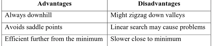
23 Thus, it can be noted that if the learning rate becomes too large, the algorithm will be unstable. If the learning rate is fixed too small, the algorithm will take a long time to converge. Highlighted in Table 2.1 are the advantages and disadvantages of this method.
Table 2.1. Advantages and Disadvantages of Gradient Descent Back-propagation (Lahmiri, 2011; Tongli et al., 2013)
Advantages Disadvantages
Always downhill Might zigzag down valleys
Avoids saddle points Linear search may cause problems Efficient further from the minimum Slower close to minimum
2.7.2 Gradient Descent with Momentum (GDM)
The back-propagation with momentum algorithm (GDM) has been largely analyzed in the neural network literature and even compared with other methods which are often trained by the use of gradient descent with momentum. A momentum term is usually included in the simulations of connectionist learning algorithms. It is well known that such a term greatly improves the speed of learning, where the momentum is used to speed up and stabilize the training iteration procedure for the gradient method. A momentum term is often added to the increment formula for the weights, in which the present weight updating increment is a combination of the present gradient of the error function and the previous weight updating increment.
The momentum parameter is analogous to the mass of Newtonian particles that moves through a viscous medium in a conservative force field. GDM depends on two training parameters. The parameter learning rate is similar to the simple gradient descent. The parameter momentum is the momentum constant that defines the amount of momentum, as in Equation 2.15.
∆𝑤𝑖𝑗(𝑟) = 𝜂 .𝛿𝑗 . 𝑥𝑖𝑗+𝛼 .∆𝑤𝑖𝑗(𝑟 −1) (2.15)
The following section describes the importance of pre-processing technique selection for classification problem, as it affects the performance of learning in Neural Network.
2.8 Data Pre-processing
Data mining is one of the most important and useful technology in the world today for extracting useful knowledge in large collections of dataset. Most of the organizations are having a large number of dataset but to extract useful and important knowledge is very difficult, and extracting knowledge without violation such as privacy and non-discrimination is most difficult and challenging (Singh & Sane, 2014). On the other hand, datasets are often large, relational and dynamic. They contain many records, places, things, events and their interactions over time. Such datasets are rarely structured appropriately for knowledge discovery, and they often contain variables whose meanings change across different subsets of the data (Fast et al., 2007).
REFERENCES
Abraham, A. (2005). Artificial neural networks. handbook of measuring system
design.
Aljawfi, O. M., Nawi, N. M., & Hamid, N. A. Enhancing Back propagation Neural
Network with Second Order Conjugate Gradient Method for Fast
Convergence.
Badri, L. (2010). Development of Neural Networks for Noise Reduction. Int. Arab J.
Inf. Technol., 7(3), 289-294.
Baskar, S. S., Arockiam, L., & Charles, S.(2013). A Systematic Approach on Data
Pre-processing In Data Mining. An international Journal of Advanced
Computer Technology (IJACT), 2, 2320-0790.
Basu, J. K., Bhattacharyya, D., & Kim, T. H. (2010). Use of artificial neural network
in pattern recognition. International journal of software engineering and its
applications, 4(2).
Beim G. P., & Wright, J. (2011). From McCulloch–Pitts Neurons Toward
Biology. Bulletin of mathematical biology, 73(2), 261-265.
Bhuiyan, M. Z. A. (2009). An algorithm for determining neural network architecture
using differential evolution. In Business Intelligence and Financial
Engineering, 2009. BIFE'09. International Conference (pp. 3-7). IEEE.
Brunette, E. S., Flemmer, R. C., & Flemmer, C. L. (2009). A review of artificial
intelligence. In ICARA (pp. 385-392).
Burr, D. J. (1988). Speech recognition experiments with perceptrons. NIPS, vol. 0,
pp. 144-153.
Chandra, P., & Singh, Y. (2004). A case for the self-adaptation of activation
functions in FFANNs. Neurocomputing, 56, pp. 447-454.
Chittineni, S., & Bhogapathi, R. B. (2012). A Study on the Behavior of a Neural
Coetzee, F. M., & Stonick, V. L. (1996). On the uniqueness of weights in
single-layer perceptrons. Neural Networks, IEEE Transactions on, 7(2), pp.
318-325.
Dan, Z. (2013). Improving the accuracy in software effort estimation: Using.
artificial neural network model based on particle swarm optimization.
InService Operations and Logistics, and Informatics (SOLI), 2013 IEEE
International Conference on (pp. 180-185). IEEE.
De Houwer, J., Barnes-Holmes, D., & Moors, A. (2013). What is learning? On the
nature and merits of a functional definition of learning. Psychonomic bulletin
& review, 20(4), pp. 631-642.
Dohnala, V., Kučab, K., & Junb, D. (2005). What are artificial neural networks and
what they can do?. Biomed Pap Med Fac Univ Palacky Olomouc Czech
Repub, 149(2), pp.221-224.
Faiedh, H., Souani, C., Torki, K., & Besbes, K. (2006). Digital hardware.
implementation of a neural system used for nonlinear adaptive prediction.
Journal of Computer Science, 2(4), pp. 355.
Fast, A., Friedland, L., Maier, M., Taylor, B., Jensen, D., Goldberg, H. G., &
Komoroske, J. (2007). Relational data pre-processing techniques for
improved securities fraud detection. In Proceedings of the 13th ACM
SIGKDD international conference on Knowledge discovery and data mining,
pp. 941-949. ACM.
Filimon, D. M., & Albu, A. (2014). Skin diseases diagnosis using artificial neural
networks. In Applied Computational Intelligence and Informatics (SACI),
2014 IEEE 9th International Symposium on (pp. 189-194). IEEE.
Fletcher, L., Katkovnik, V., Steffens, F. E., & Engelbrecht, A. P. (1998). Optimizing
the number of hidden nodes of a feedforward artificial neural network.
In Neural Networks Proceedings, 1998. IEEE World Congress on
Computational Intelligence. The 1998 IEEE International Joint Conference,
2, pp. 1608-1612.
Gao, N., & Gao, C. Y. (2010). Combining the genetic algorithms with BP Neural
Network for GPS height Conversion. In Computer Design and Applications
(ICCDA), 2010 International Conference, 2, pp. V2-404. IEEE.
60
Ghazali, R., Hussain, A. J., Al-Jumeily, D., & Lisboa, P. (2009). Time series
prediction using dynamic ridge polynomial neural networks. In Developments
in eSystems Engineering (DESE), 2009 Second International Conference
on (pp. 354-363). IEEE.
Ghwanmeh, S., Mohammad, A., & Al-Ibrahim, A. (2013). Innovative Artificial
Neural Networks-Based Decision Support System for Heart Diseases
Diagnosis.
Gudadhe, M., Wankhade, K., & Dongre, S. (2010). Decision support system for heart
disease based on support vector machine and artificial neural network.
In Computer and Communication Technology (ICCCT), 2010 International
Conference on (pp. 741-745). IEEE.
Gupta, M., & Aggarwal, N. (2010). Classification techniques analysis. In
NCCI2010-National Conference on Computational Instrumentation, CSIO Chandigarh,
India (pp. 19-20).
Gupta, S. (2013). Using artificial neural network to predict the compressive strength
of concrete containing Nano-Silica. Civil Engineering and Architecture, 1(3),
96-102.
Günther, F., & Fritsch, S. (2010). Neuralnet: Training of Neural Networks. The R
journal, 2(1), pp. 30-38.
Halder, A., Ghosh, A., & Ghosh, S. (2011). Supervised and unsupervised landuse
map generation from remotely sensed images using ant based
systems. Applied Soft Computing, 11(8), 5770-5781.
Hamid, N. A., Nawi, N. M., Ghazali, R., & Salleh, M. N. M. (2011). Improvements of Back Propagation Algorithm Performance by Adaptively Changing Gain, Momentum and Learning Rate. International Journal of New Computer Architectures and their Applications (IJNCAA), 1(4), pp. 866-878.
Hinton, G. (2003). The ups and downs of Hebb synapses. Canadian
Psychology/Psychologie canadienne, 44(1), pp. 10.
Illingworth, W. T. (1989). Beginner's guide to neural networks. InAerospace and
Electronics Conference, 1989. NAECON 1989., Proceedings of the IEEE
1989 National (pp. 1138-1144). IEEE.
Isa, I. S., Omar, S., Saad, Z., & Osman, M. K. (2010). Performance comparison of
different multilayer perceptron network activation functions in automated
Simulation (AMS), 2010 Fourth Asia International Conference on (pp.
71-75). IEEE.
Isa, I. S., Saad, Z., Omar, S., Osman, M. K., Ahmad, K. A., & Sakim, H. M. (2010).
Suitable MLP network activation functions for breast cancer and thyroid
disease detection. In Computational Intelligence, Modelling and Simulation
(CIMSiM), 2010 Second International Conference on (pp. 39-44). IEEE.
Jabbar, M. A., Deekshatulu, B. L., & Chandra, P. (2013). Heart Disease Prediction
System using Associative Classification and Genetic Algorithm. arXiv
preprint arXiv:1303.5919
Jayalakshmi, T., & Santhakumaran, A. (2011). Statistical normalization and back
propagation for classification. International Journal of Computer Theory and
Engineering, 3(1), 1793-8201.
Jin, L. V., Guo, C., Shen, Z. P., Zhao, M., & Zhang, Y. (2007). Summary of
Artificial Neuron Model Research. In Industrial Electronics Society, 2007.
IECON 2007. 33rd Annual Conference of the IEEE (pp. 677-682). IEEE.
Kamruzzaman, J., & Aziz, S. M. (2002). A note on activation function in multilayer
feedforward learning. In Neural Networks, 2002. IJCNN'02. Proceedings of
the 2002 International Joint Conference, 1, pp. 519-523. IEEE.
Kaur, A., Monga, H., & Kaur, M. (2012). Performance Evaluation of Reusable
Software Components. International Journal of Emerging Technology and
Advanced Engineering, 2(4).
Kaur, T. (2012). Implementation of Backpropagation Algorithm: A Neural Net-work
Approach for Pattern Recognition. International Jounal of Engineering
Reasearch and Development, 1(5), 30-37.
Khemphila, A., & Boonjing, V. (2010). Comparing performances of logistic
regression, decision trees, and neural networks for classifying heart disease
patients. In Computer Information Systems and Industrial Management
Applications (CISIM), 2010 International Conference on, (pp. 193-198).
Khemphila, A., & Boonjing, V. (2011). Heart disease classification using neural
network and feature selection. In Systems Engineering (ICSEng), 2011 21st
International Conference on (pp. 406-409). IEEE.
62
Koskivaara, E. (2000). Different pre-processing models for financial accounts when
using neural networks for auditing. ECIS 2000 Proceedings, 3.
Krenker, A., Kos, A., & Bešter, J. (2011). Introduction to the artificial neural
networks. INTECH Open Access Publisher.
Lahmiri, S. (2011). A comparative study of backpropagation algorithms in financial
prediction. International Journal of Computer Science, Engineering and
Applications (IJCSEA), 1(4).
Lee, S. W., & Moraga, C. (1996). A Cosine-Modulated Gaussian activation function
for Hyper-Hill neural networks. In Signal Processing, 1996., 3rd
International Conference, 2, pp. 1397-1400. IEEE.
Lei, S., & Xing-cheng, W. (2010). Artificial neural networks: current applications in
modern medicine. In Computer and Communication Technologies in
Agriculture Engineering (CCTAE), 2010 International Conference, 2, pp.
383-387. IEEE.
Leung, F. H. F., Lam, H. K., Ling, S. H., & Tam, P. K. S. (2003). Tuning of the
structure and parameters of a neural network using an improved genetic
algorithm. Neural Networks, IEEE Transactions on, 14(1), pp.79-88.
Li, H., Yang, D., Chen, F., Zhou, Y., & Xiu, Z. (2014). Application of Artificial
Neural Networks in predicting abrasion resistance of solution polymerized
styrene-butadiene rubber based composites. In Electronics, Computer and
Applications, 2014 IEEE Workshop on (pp. 581-584). IEEE.
Liu, H. X., Zhang, R. S., Luan, F., Yao, X. J., Liu, M. C., Hu, Z. D., & Fan, B. T.
(2003). Diagnosing breast cancer based on support vector machines. Journal
of chemical information and computer sciences, 43(3), pp. 900-907.
Magoulas, G. D., Plagianakos, V. P., & Vrahatis, M. N. (2000). Development and
convergence analysis of training algorithms with local learning rate
adaptation. In Neural Networks, IEEE-INNS-ENNS International Joint
Conference on, 1, pp. 1021-1021. IEEE Computer Society.
Mali, S. B. (2013). Soft Computing on Medical-Data (SCOM) for a Countrywide
Medical System Using Data Mining and Cloud Computing Features. Global
Journal of Computer Science and Technology, 13(3).
Mantzaris, D., Vrizas, M., Trougkakos, S., Priska, E., & Vadikolias, K. (2014).
Artificial Neural Networks for Estimation of Dementias Types. Artificial
Mathis, H., von Hoff, T. P., & Joho, M. (2001). Blind separation of signals with
mixed kurtosis signs using threshold activation functions. Neural Networks,
IEEE Transactions on, 12(3), 618-624.
Mazurowski, M. A., Habas, P. A., Zurada, J. M., Lo, J. Y., Baker, J. A., & Tourassi,
G. D.(2008). Training neural network classifiers for medical decision
making: The effects of imbalanced datasets on classification performance.
Neural networks, 21(2), 427-436.
Mazurowski, M. A., Zurada, J. M., & Tourassi, G. D. (2008). Selection of examples
in case-based computer-aided decision systems. Physics in medicine and
biology, 53(21), 6079.
Miksovsky, P., Matousek, K., & Kouba, Z. (2002). Data pre-processing support for
data mining. In Systems, Man and Cybernetics, 2002 IEEE International
Conference on, 5, pp. 4-pp. IEEE.
Mitrea, C. A., Lee, C. K. M., & Wu, Z. (2009). A comparison between neural
networks and traditional forecasting methods: A case study. International
Journal of Engineering Business Management, 1(2), 19-24.
Modugno, R., Pirlo, G., & Impedovo, D. (2010). Score normalization by dynamic
time warping. In Computational Intelligence for Measurement Systems and
Applications (CIMSA), 2010 IEEE International Conference on, (pp. 82-85).
IEEE.
Mokhlessi, O., Rad, H. M., & Mehrshad, N. (2010). Utilization of 4 types of
Artificial Neural Network on the diagnosis of valve-physiological heart
disease from heart sounds. In Biomedical Engineering (ICBME), 2010 17th
Iranian Conference of , (pp. 1-4). IEEE.
Nakayama, K., & Ohsugi, M. (1998). A simultaneous learning method for both
activation functions and connection weights of multilayer neural networks.
In Proc. IJCNN, 98, pp. 2253-2257.
Nayak, S.C., Misra, B.B. and Behera, H.S. (2014). Impact of Data Normalization on Stock Index Forecasting International Journal of Computer Information Systems and Industrial Management Applications. 6, 357-369.
Nawi, N. M., Khan, A., & Rehman, M. Z. (2013). A New Levenberg Marquardt
Based Back Propagation Algorithm Trained with Cuckoo Search. Procedia
64
Nawi, N. M., Atomi, W. H., & Rehman, M. Z. (2013). The Effect of Data
Pre-processing on Optimized Training of Artificial Neural Networks. Procedia
Technology, 11, 32-39.
Nicoletti, G. M. (1999). Artificial neural networks (ANN) as simulators and
emulators-an analytical overview. In Intelligent Processing and
Manufacturing of Materials, 1999. IPMM'99. Proceedings of the Second
International Conference on, 2, pp. 713-721. IEEE.
Ogasawara, E., Martinez, L. C., de Oliveira, D., Zimbrão, G., Pappa, G. L., &
Mattoso, M. (2010). Adaptive normalization: A novel data normalization
approach for non-stationary time series. In Neural Networks (IJCNN), The
2010 International Joint Conference on (pp. 1-8). IEEE.
Ozcan, H. K., Ucan, O. N., Sahin, U., Borat, M., & Bayat, C. (2006). Artificial
neural network modeling of methane emissions at Istanbul
Kemerburgaz-Odayeri Landfill Site. Journal of scientific and industrial research, 65(2),
128.
Özkan, C., & Erbek, F. S. (2003). The comparison of activation functions for
multispectral Landsat TM image classification. Photogrammetric
Engineering & Remote Sensing, 69(11), 1225-1234.
Pattichis, C. S., & Pattichis, M. S. (2001). Adaptive neural network imaging in
medical systems. In Signals, Systems and Computers, 2001. Conference
Record of the Thirty-Fifth Asilomar Conference on, 1, pp. 313-317.IEEE.
Penedo, M. G., Carreira, M. J., Mosquera, A., & Cabello, D. (1998). Computer-aided
diagnosis: a neural-network-based approach to lung nodule detection.Medical
Imaging, IEEE Transactions on, 17(6), 872-880.
Perumal, K., & Bhaskaran, R. (2010). Supervised classification performance of
multispectral images. arXiv preprint arXiv:1002.4046.
Piekniewski, F., & Rybicki, L. (2004). Visual comparison of performance for
different activation functions in MLP networks. In Proceedings of
International Joint Conference on Neural Networks: IJCNN, 4(4), pp.
2947-2952).
Pierrehumbert, J. B., Stonedahl, F., & Daland, R. (2014). A model of grassroots
changes in linguistic systems. arXiv preprint arXiv:1408.1985.
Pourmohammad, A., & Ahadi, S. M. (2009). Using single-layer neural network for
Communications and Signal Processing, 2009. ICICS 2009. 7th International
Conference on, (pp. 1-4). IEEE.
Psichogios, D. C., & Ungar, L. H. (1992). A hybrid neural network‐first principles
approach to process modeling. AIChE Journal, 38(10), 1499-1511.
Razavi, S., & Tolson, B. A. (2011). A new formulation for feedforward neural
networks. Neural Networks, IEEE Transactions on, 22(10), pp.1588-1598.
Rehman, M. Z., & Nawi, N. M. (2011). Improving the Accuracy of Gradient Descent
Back Propagation Algorithm (GDAM) on Classification Problems.
International Journal of New Computer Architectures and their Applications
(IJNCAA), 1(4), pp. 838-847.
Richiardi, J., Achard, S., Bunke, H., & Van De Ville, D. (2013). Machine learning
with brain graphs: predictive modeling approaches for functional imaging in
systems neuroscience. Signal Processing Magazine, IEEE, 30(3), pp. 58-70.
Robinson, A. J., & Failside, F. (1988). Static and dynamic error propagation
networks with application to speech coding. In Neural information
processing systems (pp. 632-641).
Roodposti, E. R., & Rasi, R. E. (2011). Sensitivity Analysis based on Artificial
Neural Networks for Evaluating Economical Plans. In Proceedings of the
World Congress on Engineering, 1, pp. 6-8.
Seung, S. (2002). Multilayer perceptrons and backpropagation learning. 9.641
Lecture4, pp.1-6.
Shin-ike, K. (2010). A two phase method for determining the number of neurons in
the hidden layer of a 3-layer neural network. In SICE Annual Conference
2010, Proceedings of (pp. 238-242).IEEE.
Shouman, M., Turner, T., & Stocker, R. (2012). Using data mining techniques in
heart disease diagnosis and treatment. In Electronics, Communications and
Computers (JEC-ECC), 2012 Japan-Egypt Conference on, pp. 173-177.
IEEE.
Sibi, M. P., Ma, Z., & Jasperse, C. P. (2005). Enantioselective addition of nitrones to activated cyclopropanes. Journal of the American Chemical Society, 127(16), 5764-5765.
Sibi, P., Jones, S. A., & Siddarth, P. (2013). Analysis Of Different Activation
Functions Using Back Propagation Neural Networks. Journal of Theoretical
66
Singh, J., & Sane, S. S. (2014). Preprocessing Technique for Discrimination
Prevention in Data Mining.
Svozil, D., Kvasnicka, V., & Pospichal, J. (1997). Introduction to multi-layer
feed-forward neural networks. Chemometrics and intelligent laboratory systems,
39(1), pp. 43-62.
Tsai, D. Y., Watanabe, S., & Tomita, M. (1996). Computerized analysis for
classification of heart diseases in echocardiographic images. In Image
Processing, 1996. Proceedings., International Conference on, 3, pp. 283-286.
IEEE.
Tongli, L., Minxiang, X., Jiren, X., Ling, C., & Huaihui, G. (2013). Modified BP
neural network model is used for oddeven discrimination of integer number.
In Optoelectronics and Microelectronics (ICOM), 2013 International
Conference on (pp. 67-70). IEEE.
Vogl, T. P., Mangis, J. K., Rigler, A. K., Zink, W. T., & Alkon, D. L. (1988).
Accelerating the convergence of the back-propagation method. Biological
cybernetics, 59(4-5), pp. 257-263.
Wanas, N., Auda, G., Kamel, M. S., & Karray, F. A. K. F. (1998). On the optimal
number of hidden nodes in a neural network. In Electrical and Computer
Engineering, 1998. IEEE Canadian Conference on, 2, pp. 918-921. IEEE.
Wentao, H. U. A. N. G., & Youceng, F. E. N. G. (2011). Small-world properties of
human brain functional networks based on resting-state functional MRI.
Journal of Huazhong Normal University (Natural Sciences), 4, 011.
Wong, K. W., Leung, C. S., & Chang, S. J. (2002). Use of periodic and monotonic
activation functions in multilayer feedforward neural networks trained by
extended Kalman filter algorithm. In Vision, Image and Signal Processing,
IEE Proceedings, 149(4), pp. 217-224. IET.
Xie, Z. (2012). A non-linear approximation of the sigmoid function based on FPGA.
In Advanced Computational Intelligence (ICACI), 2012 IEEE Fifth