Munich Personal RePEc Archive
On the Existence and Stability of Pareto
Optimal Endogenous Matching with
Fairness
Dai, Darong
Department of Economics, School of Business, Nanjing University
8 August 2012
ON THE EXISTENCE AND STABILITY OF PARETO OPTIMAL
ENDOGENOUS MATCHING WITH FAIRNESS
Darong Dai
Department of Economics, School of Business, Nanjing University, Nanjing 210093,
P. R. China
E-mail:
[email protected]
.
Abstract
In the current paper, we study the asymmetric normal-form game between two heterogeneous groups of populations by employing the stochastic replicator dynamics driven by Lévy process. A new game equilibrium, i.e., the game equilibrium of a stochastic differential cooperative game on time, is derived by introducing optimal-stopping technique into evolutionary game theory, which combines with the Pareto optimal standard leads us to the existence of Pareto optimal endogenous matching. Moreover, stability of the Pareto optimal endogenous matching is confirmed by essentially using the well-known Girsanov Theorem.
Keywords:
Stochastic differential cooperative game on time; Endogenous matching;
Stability; Fairness; Adaptive learning.
JEL
classification:
C62; C70; C78.
It is convincing to argue that people live in a highly structured society consists of groups rather than individuals, which implies that random matching will not always provide us with compelling approximation to reality when we are concerned with the interactions among the players. In fact, Ellison (1993) shows that local interaction will have very important and also different implications in equilibrium selection relative to that of uniform interaction or random matching. So, given the importance of non-random matching in equilibrium selection, we express the motivation of the present paper as follows, i.e., can we directly prove the existence and stability of certain non-random matching that is Pareto optimal and also endogenously determined in a given game situation? If we can, what are the conditions we will rely on? In other words, the major goal of the present exploration is not to study any exogenously given matching mechanism but to find out the optimal matching mechanism in a given game situation, and to prove its stability.1
In two pioneering papers, Kandori et al. (1993) and Young (1993) prove that the trial-and-error learning processes of the players will definitely converge to one particular pure-strategy Nash equilibrium, which is named as the long run equilibrium by Kandori et al. and the convention by Young. From the perspective of multiple-equilibrium problem, they provide us with an equilibrium selection device, under which the players are correctly predicted to play a particular Nash equilibrium. However, we can also evaluate their contribution from the following view of point, i.e., provided a particular Nash equilibrium, they prove that there exists a pattern of learning mechanism that will definitely lead the players to play the given Nash equilibrium. To summarize, they confirm the existence of certain type of learning mechanism, based upon which the players’ behavior will be uniquely predicted in the long run. Instead of emphasizing micro-strategy, we focus on macro-structure
and it is confirmed that there exist certain macro-structure under which one particular Pareto optimal Nash equilibrium will be definitely played by the players. Obviously, in order to derive much more comprehensive understanding of the strategic behaviors of the individuals in a given society, micro-strategy and macro-structure should be explored as a whole. Accordingly, the present study also examines the internal relationship between the micro-strategy and the macro-structure by analyzing the internal relationship between the learning mechanism and the matching mechanism. That is to say, the Pareto optimal endogenous matching as well as the Pareto-optimal Nash equilibrium can be regarded as the limit of the learning processes of the players in some sense by noting that there exists a one-to-one correspondence between the Pareto optimal endogenous matching and the Pareto optimal Nash equilibrium. Furthermore, if we argue that different matching mechanisms imply different Nash equilibria, we have demonstrated that there exists certain learning mechanism under which one particular matching mechanism will be achieved, that is, one particular micro-strategy implies one particular macro-structure under certain relatively weak conditions. To conclude, we indeed prove the following two important and also interesting claims: first, provided a particular Nash equilibrium, we show the existence of one matching mechanism such that the given
Nash equilibrium will be endogenously chosen by the players as a rational prediction; second, given a particular matching mechanism, we demonstrate the existence of certain learning mechanism so that the given matching mechanism will be endogenously established by all the players spontaneously in the long run. We therefore believe that the present study has supplied an interesting and also relatively complete characterization of the internal relationship between the micro-strategy employed by the players and the macro-structure facing the players.
In the paper, we are encouraged to study the asymmetric normal-form games between two heterogeneous groups of populations under the modified framework of evolutionary game theory.2
Each of the two groups is assumed to have countable many pure strategies. Hyper-rational assumptions (see, Aumann, 1976) about the players broadly used in classical non-cooperative game theory will be dropped in the present model, instead, the players or individuals play the game following certain adaptive learning processes arising from the stochastic replicator dynamics driven by Lévy processes for the first time.3 On the contrary, the strategies themselves are supposed to be smart and rational enough to optimize their fitness4, which directly depend on the stochastic
replicator dynamics or the learning processes of the players, following the classical as if methodology from the perspective of posteriori. And the corresponding control variables of these fitness- optimization problems5 are chosen to be stochastic stopping times or stopping rules, which reasonably reflects the fact that strategies themselves are no longer suitable for the roles of control variables as in the best-response correspondences of Nash equilibria because “strategies” of the players’ strategies will not be well-defined through the traditional approach. Luckily, noting that the optimal stopping rules are partially determined and completely characterized by the learning processes of the players, the optimal stopping rules as a whole may be exactly one of the Nash equilibra, no matter it is a mixed-strategy Nash equilibrium or a pure-strategy Nash equilibrium, of the original normal-form games derived from the best-response approach.6 Generally speaking, the
2 It will be without loss of nay generality when focusing on the case of two heterogeneous groups of populations by noting that two-sided markets broadly exist in reality, for instance, the marriage market and the labor market.
3 We extend the pioneering stochastic replicator dynamics of Foster and Young (1990) and Fudenberg and Harris (1992) to Lévy processes by emphasizing the role of jumps in learning processes. Binmore and Samuelson (1999) show the importance of drift in equilibrium selection, and here we point out that jumps not only really happen in social and biological evolution but also play crucial role in equilibrium selection.
4 We prefer fitness to payoff because payoff will neglect some important and even determinant factors in equilibrium selection. Fitness will be a much more complete characterization of the objective of the player than payoff. Fitness not only focuses on the game itself like payoff but also pays attention to other factors, such as the environment where the game happens and also the importance of the game to the players by noting that players usually are faced with many different or alternative games at the same time, which often leads to the fact that there exist substitutive and complementary relationship between these games from the perspective of the players, thereby violating the usually implicit assumption that each game is regarded as an isolated one. To sum up, the concept of fitness will capture much more relevant factors of the game situations facing the players, including objective factors like payoff structure and also subjective factors like the degree of game participation.
5 In the current model, we do not incorporate inter-temporal consideration like that of Matsui and Matsuyama (1995) into the present optimization problem because we insist that the present case is of independent interest.
optimal stopping rules as a whole will not be equal to anyone of the Nash equilibria, that is, there exists certain difference between the both. However, it is confirmed that it is just the difference between the optimal stopping rules as a whole and the Pareto optimal Nash equilibrium of the original normal-form game that established our Pareto optimal endogenous matching. We, hence, to the best of our knowledge, enrich the matching rule widely used in evolutionary game theory by naturally adding into economic-welfare implications for the first time.7
Moreover, it is shown that the well-known random matching (e.g., Maynard Smith, 1982; Fudenberg and Levine, 1993; Ellison, 1994; Okuno-Fujiwara and Postlewaite, 1995; Weibull, 1995) just represents one special and extreme case of the current endogenous matching and we supply the conditions under which the random matching will be asymptotically Pareto efficient.8 Thus, proving the
existence of Pareto optimal endogenous matching would be regarded as one innovation of the present paper by noticing the above facts.
Up to the present step of our story, we have been provided with a Pareto-optimal endogenous matching in the current game situation by solving the above fitness-optimization problems of the
limiting distribution, i.e., sending the number of population to infinity, sending the time to infinity or sending the mistakes to zero, and we finally compare it with the classical solution concept like Nash equilibrium. Therefore, if we argue that the traditional approach focuses on strategy-space dimension, evolutionary game theory pays relatively more attention to evolutionary-time dimension (see, Binmore and Samuelson, 1997, 1999; Binmore et al., 1995). Evolutionary game theory prefers to study the basin of attraction (see, Ellison, 2000), the steady state (Fudenberg and Levine, 1993) or the rest point of the evolutionary dynamics or learning processes, we argue that optimal stopping rule plays the similar role except that rest point of dynamics only depends on the properties of the dynamics themselves while optimal stopping rule adding into a rational constraint. To summarize, the traditional approach emphasizes
micro-strategy from the perspective of individual choice while evolutionary game theory focuses more on macro-structure from the viewpoint of group evolution, and the method introduced in the present paper will supply a linkage between the both, that is to say, optimal stopping rule is partially determined and completely characterized by macro-structure while it is also partially determined by micro-strategy.
7 Existing studies usually focus on the enforcement or reputation mechanism for given matching mechanism (see, Kandori, 1992, for instance). Then they explore the corresponding welfare implications of the enforcement or reputation mechanism. We, however, directly examine the welfare implications of the matching mechanism by noting that it will lead us to the Pareto efficient equilibrium. 8 For any given game, different matching patterns imply different payoffs for the players. Rather, if we let the payoffs corresponding to random matching, which does work in a perfect world with well-mixed population, denote the benchmark, the payoffs defined by any non-random matching would be regarded as certain perturbations to the benchmark-payoffs by noting the linearity of von Neuman-Morgenstern payoff functions. And in this sense, we argue that random matching just represents a special case where we have sent the payoff- perturbations to zero. However, why we argue that non-random matching, especially endogenous matching, is of crucial importance? Besides the argument of Ellison (1993), we point out the following problem, that is, random matching usually leads the dynamics or learning processes to equilibrium that is not Pareto efficient and even Pareto inefficient (see, Weibull, 1995, for instance). Consequently, in order to prevent the dynamics or learning processes from being attracted into the Pareto inefficient rest point, we introduce mutations or perturbations into the dynamics or the learning processes to produce efficient equilibrium (see, Canning, 1992; Binmore and Samuelson, 1999). And we show that non-random matching mechanism will be a suitable choice. Furthermore, it is easily noticed that most of the existing literatures (see, Fudenberg and Levine, 1993; Kandori et al., 1993; Young, 1993, and among others) employ the random matching to study the game played by a large population of players, however, for the games in reality, random matching is much more suitable for the case that consists of small population of players, for example, in a village or in a community. Let us consider a gift-giving game in a village or in a community, and it is reasonably to suppose that the players will interact with each other equally thanks to the reputation effect or enforcement effect. Now, let us consider the same gift-giving game with the players coming from two isolated villages or communities, we can easily find that the interacting frequency in each village or community will be much higher than that between the two villages or communities. That is to say, this is an imperfect world and people live in a highly structured society. To sum up, if we study the game played by a small population of players, random matching really works, however, if we study the game played by a large population of players, random matching should not be directly applied to the whole population, and the population should be divided into many sub-populations (see, Young (1993)) and we apply random matching to each sub-population while non-random matching will be suitable for the interactions between these
strategies and then smoothing the possible or potential difference between the corresponding optimal stopping rules as a whole and the Pareto optimal Nash equilibrium of the original normal-form game. In other words, the Pareto optimal Nash equilibrium of the original asymmetric normal-form game can be actually achieved by the two heterogeneous groups of populations as a rational solution of the above fitness-optimization problems given the existence of the Pareto optimal endogenous matching. Now, we proceed to the next step of demonstrating the stability of the Pareto optimal matching given its existence. Noting that there exists a one-to-one correspondence between the Pareto optimal matching and the Pareto optimal Nash equilibrium, we then just need to prove the stability of the Pareto optimal Nash equilibrium, and also it will be confirmed that this equivalent transformation will apparently and greatly lower the technical requirement. Indeed, we prove that the adaptive learning processes will uniformly and robustly converge to the above Pareto optimal Nash equilibrium as the time approaching infinity while the errors or stochastic perturbations in the learning processes always exist except that they are reasonably controlled in certain region following from the martingale property. That is to say, the learning processes will robustly converge to the modified9 optimal stopping rules as a whole, i.e., the Pareto optimal Nash equilibrium, in the sense
of uniform topology as long as the adaptive learning processes exhibit martingale property, which, however, can be established by applying the well-known Girsanov Theorem under certain weak conditions10. Accordingly, the present paper not only proves the stability of the Pareto optimal
endogenous matching but also confirms the following important and also interesting byproduct, i.e., we claim: the adaptive learning processes of the individuals will uniformly and robustly converge to the Pareto optimal Nash equilibrium, which is exactly the rational solution of the above fitness-optimization problems of the strategies given the Pareto optimal endogenous matching, of the original normal-form game as long as they exhibit martingale property.11 We, hence, argue that
this conclusion would be regarded as one major contribution of the current study when compared with existing literatures, for example, first, existing literatures12 (see, Canning, 1992; Young, 1993;
Kandori et al., 1993) proved the similar convergence essentially requiring that the errors or perturbations approach zero; second, existing literatures showed that their learning processes will either converge to a mixed-strategy Nash equilibrium (e.g., Fudenberg and Kreps, 1993; Benaïm and
9 It is modified by the Pareto optimal endogenous matching. 10 That is, the Novikov conditions are assumed to be fulfilled.
11 What’s the aspiration of this conclusion? We emphasize the following three points: first, endogenous matching mechanism will meet the gap between the Pareto optimal Nash equilibrium and the limiting behavior of evolutionary dynamics or adaptive learning processes, and this Pareto optimal endogenous matching mechanism is exactly the matching mechanism that requires the least information, especially in computation; second, one can directly model stochastic learning processes with martingale property in future research; finally, our argument is in line with some of the existing studies (see, Harsanyi, 1973; Canning, 1992; Fudenberg and Kreps, 1993; Binmore and Samuelson, 1999) by noting that martingale process itself is a stochastic process, i.e., there exist persistent stochastic perturbations in the corresponding learning processes and hence the payoffs.
Hirsch, 1999; Ellison and Fudenberg, 2000, and among others) or a pure-strategy Nash equilibrium (see, Young, 1993; Kandori et al., 1993) depending on the types of learning processes they specified13
while the current exploration confirms that convergence always happens under weak conditions and also the limit will be a Pareto optimal Nash equilibrium given the endogenous matching mechanism, thus, we supply a unified framework by introducing the endogenous matching; third, convergence of the learning processes not only implies the Pareto-dominant equilibrium in coordination games but can also yield cooperation equilibrium in PD games by slightly modifying the endogenous matching mechanism,14 which reflects that matching mechanism as well as learning mechanism should be paid
at least equal attention to in our study;15 forth, the convergence result implicitly argues that the learning approach need not to be absolutely different from the traditional rational-approach, otherwise, we can tell why the difference exists and what forms the difference, and finally we demonstrate that the endogenous matching mechanism will provide us with a practical bridge that links the learning approach and the traditional approach, thereby effectively meeting the so-called unbridgeable gap; last but not least, our robust convergence happens in a persistently non-stationary environment and in the sense of uniform topology, and hence it is obviously much stronger than that of existing studies (see, Kandori et al., 1993; Young, 1993; Fudenberg and Kreps, 1993; Benaïm and Hirsch, 1999) after a quick check.
Although the major contribution of the present limited study has been expressed above, the following innovations are also worth noticing in some sense. Indeed, the existence and stability of the Pareto optimal endogenous matching are not necessarily independent of each other. For instance, on the one hand, one can easily find that the stability assertion intimately depends on the characterization of the existence result by checking the details of the following proof in Appendix C.16 On the other hand, the expected fitness of the strategies will also exhibit martingale property if
the corresponding adaptive learning processes are martingale processes by noting the mathematical conclusion that martingale property keeps invariant under affine transformation. To conclude, stability produces existence in turn in the following sense, i.e., stability of the Pareto optimal endogenous matching implies the existence of Pareto optimal matching with fairness because the game between different strategies will become a fair-game after the martingale-payoffs being incorporated into the game-situations. And this is why the word “fairness” specifically appears in the title of the paper.
13 For example, one major difference between Fudenberg and Kreps’s (1993) model and Young’s (1993) model is that Fudenberg and Kreps use a generalization of fictitious play where the players asymptotically choose the best replies to other players’ past actions based upon the entire historical frequencies, while the players base their decisions on limited information in Young’s model. Moreover, in contrast to the model of Fudenberg and Kreps, the players do not always optimize in Young’s model.
14 Noting that the risk-dominant equilibrium usually has a larger basin of attraction than the Pareto dominant equilibrium, and both-defect is the only Nash equilibrium in PD games, the endogenous matching mechanism truly plays a key role in equilibrium selection.
15 It is compelling that matching mechanism would be regarded as an equilibrium selection device in some sense. Indeed, the current study is concerned with the case that matching leads to unique equilibrium. Moreover, the stability of the matching mechanism implies the stability of the equilibrium selection.
Furthermore, the present paper defines a much stronger stability concept of equilibrium strategy and hence matching pattern by naturally combining the traditional interpretation and the evolutionary interpretation. Because the strategies are proposed to be as if rational “players” in some sense, it is easily discovered below that the optimal stopping rules as a whole is computed by satisfying the following two constraints, i.e., individually-rational solution and no blocks exist17, which implies certain stability from the concept of Nash bargaining solution (see, Nash, 1950) in cooperative game theory. However, we do not stop here by just focusing on rational requirements of stability from the viewpoint of micro-strategy. We also emphasize the importance of evolutionary interpretation from the group level as a whole, i.e., the macro-structure. We do this by building up new adaptive-learning processes via introducing exogenous perturbations into the original learning processes, and we prove that the new learning processes and the original learning processes will converge to the same equilibrium as the exogenous perturbations approaching zero. We should specifically emphasize that the original learning processes themselves are driven by Lévy processes, i.e., including both diffusion terms and jump terms. Thus, in order to build up new learning processes, all we have to do is to disturb the original drift terms, diffusion terms and the original jump terms. Consequently, the new adaptive learning processes are also driven by Lévy processes. To summarize, we check the stability from the viewpoint of macro-structure by not essentially changing the errors or perturbations existing in the original learning processes, and we take limit just by sending the exogenous perturbations to zero.
In the next section, some well-known examples of crucial importance in non-cooperative game theory will be presented and discussed to help capture some basic ideas and intuitions of the formal model. Section 3 will construct the formal model, introduce some basic concepts and prove the key theorem of the present paper. Section 4 is used to demonstrate the stability of the Pareto optimal endogenous matching. There is a brief concluding section. All proofs, unless otherwise noted in the text, appear in the Appendix.
2. Examples
Before constructing formal models, we will first introduce some well-known and also simple examples of non-cooperative game theory in the current section. And it is believed that these examples would help a lot in understanding the formulation in the following section and capturing the economic intuitions behind the model for the readers. Moreover, it is worth noting that these examples would have effectively reflected some ideas of the formulation, they are nevertheless far
away from representing the whole story of the current investigation. EXAMPLE 1—Classical Prisoner’s Dilemma.
Player 2 C D
[image:9.595.133.376.188.286.2]
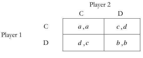
Figure 1 - Symmetric PD Game
In Figure 1, C and D are used to denote strategies cooperation and defection, respectively. And it is assumed that d a b c. As usual, the entries in the matrix represent corresponding payoffs of player 1 and player 2, respectively, for any given strategy choices. For instance, ( , )c d implies that player 1 will get payoff c if she chooses strategy C given player 2 chooses strategy D, and vice versa. And it is well known that (D, D) is the only Nash equilibrium in one-short situations and for rational players with common knowledge (see, Aumann, 1976) although (C, C) strictly Pareto dominates it. And most of excellent existing literatures have been devoted to searching for possible mechanism, i.e., enforcement mechanism18, rational mechanism19, learning mechanism20 and
evolutionary mechanism21, so that (C, C) will be actually chosen, thereby breaking through the so-called dilemma. In the current paper, we study the mechanism of endogenous matching. Indeed, one can easily note below that our approach is equivalent to that of disturbing payoff to some extent and in some sense. Noting that pure strategy stands for one special case of mixed strategy, i.e., all other pure strategies are given zero-probability weights while the chosen pure strategy with one-probability weight. Moreover, by noting the symmetry, we just consider the case that player 2 chooses to randomize his strategy choice between C and D, i.e., she chooses C with probability p
and chooses D with probability 1p with 0 p 1. Now, as the players are involved in a structured society, we introduce endogenous matching by adding to p while adding to
1p, that is to say, we get a new weighted form (p,1 p ). And we define the generalized
18 See, Fudenberg and Maskin (1986), Kandori (1992), Ellison (1994) and among others. 19 See, Kreps et al. (1982), Andreoni and Samuelson (2006).
20 See, Selten and Stoecker (1986), Kirchkamp and Nagel (2007).
21 See, Axelrod (1984), Fudenberg and Maskin (1990), Young and Foster (1991), Nowak et al. (2004), Imhof (2005), Imhof and
Nowak (2006) and among others.
Player 1
C a,a c,d
expected payoffs of player 1 by,
1(
EU C, (p,1 p ))a p( ) c(1 p )
apc(1p)
(ac),And,
1
EU (D, (p,1 p ))d p( ) b(1 p )
dpb(1p)
(d b),where (a c ) and (db) could be regarded as perturbations of the expected payoffs of strategy C and strategy D, respectively, for player 1 and provided that player 2 randomizes between strategy C and strategy D by ( ,1p p) with 0 p1. Letting EU1( C, (p, 1
))
p EU1(D, (p,1 p )), we obtain
(ad p) (c b)(1p) (
d b c a). Noting that (C, C) Pareto dominates (D, D), we put p1 and then we get the Pareto optimal endogenous matching22
( , ), ( , )
with (ad) (d b c a). And thus, we call (C, C) the induced Pareto optimal game equilibrium, i.e., an equilibrium induced by the above Pareto optimal endogenous matching
( , ), ( , )
.EXAMPLE 2—Asymmetric Prisoner’s Dilemma. Player 2 C D
[image:10.595.134.377.475.581.2]
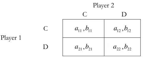
Figure 2 - Asymmetric PD Game
Noting that Figure 2 shows an asymmetric PD game, we then must have a21a11a22 a12 and
12 11 22 21
b b b b . Here we specifically study the asymmetric PD game because asymmetric games
22 One can easily tell the difference between the definition of matching in the current paper and that in existing literatures. That is to say, we use the word “matching” in a generalized fashion because our “endogenous matching” really plays similar role as that of matching usually used and understood. Moreover, one can also interpret our definition of matching in the following way, i.e., we call the “disturbance” itself that essentially induces new matching pattern as the definition of endogenous matching because we only care about the “disturbance” in most cases.
Player 1
C a11,b11 a12,b12
themselves play a very important role in non-cooperative game theory. In particular, asymmetric games usually appear in evolutionary game theory where we study the replicator dynamics of interacting heterogeneous populations in stationary or fluctuating environments23. Again, (D, D) is
the unique strictly Nash equilibrium while (C, C) Pareto (or payoff) dominates (D, D). Now, suppose that player 2 randomizes between C and D, i.e., she chooses C with probability p2 while she
employs D with probability 1p2 with 0 p2 1. And, as the players are involved in a structured
society rather than a well-mixed population, we introduce endogenous matching by adding 2 to
2
p while adding 2 to 1p2, then we get a new weighted form (p22,1p22). So, the
generalized expected payoffs of player 1 can be expressed as
1(
EU C, (p22,1p22))
11( 2 2) 12(1 2 2)
a p a p
a p11 2a12(1p2)
(a11a12)2,And,
1
EU (D, (p2 2,1p22))
21( 2 2) 22(1 2 2)
a p a p
a p21 2a22(1p2)
(a21a22)2,We then get 2(a11a21) (a21a22a12a11) by letting EU1(C,(p22,1 p2 2))EU1
(D, (p2 2,1p22)) and sending p2 to 1. Similarly, assume that player 1 randomizes
between C and D, that is, she chooses C with probability p1 and D with probability 1p1 with
1
0 p 1. We incorporate endogenous matching here by adding 1 to p1 while adding 1 to
1
1p , thereby implying a new weighted form (p11,1p11). Thus, player 2 exhibits the
following generalized expected payoffs, i.e.,
2(
EU C,(p11,1p11))b11(p11)b21(1p11)
b p11 1b21(1p1)
(b11b21)1,And,
2
EU (D,(p11,1p11))b12(p11) b22(1p11)
b p12 1b22(1p1)
(b12 b22)1,We then get 1
11 12
(b b )1 (b12b22b21b11)by letting EU2(C,(p11,1 p1 1)) EU2
(D, (p11,1 p11)) and sending p1 to 1. Consequently, we obtain the corresponding Pareto
optimal endogenous matching rule denoted
( ,1 1), ( ,2 2)
with 1
11 12 12 22 21 11
b b b b b b
and 2
11 21 21 22 12 11
(a a ) (a a a a ). And also, (C, C) can be regarded as the induced Pareto optimal game equilibrium in the current game situation.
EXAMPLE 3—Symmetric Coordination Game. Player 2 I II
[image:12.595.134.374.340.431.2]
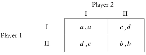
Figure 3 - Symmetric Coordination Game
We suppose that ad, bc, a d b c and ba in Figure 3. Rather, Figure 3 reveals a classical symmetric coordination game with the pure strategy space {I, II}. There are three strictly Nash equilibria in the game, i.e., two pure-strategy Nash equilibra, denoted (I, I) and (II, II), and one mixed-strategy Nash equilibrium (( ,1pˆ pˆ), ( ,1pˆ pˆ)) with ˆ b c
a c b d
p . Notice that we suppose that a d b c, which implies that equilibrium (I, I) strictly risk dominates (see, Harsanyi and Selten, 1988) equilibrium (II, II). Nonetheless, equilibrium (II, II) strictly Pareto (or payoff) dominates
equilibrium (I, I) since it is assumed that ba. Then we are faced with one of the most important issues in non-cooperative game theory, i.e., multiple-equilibrium problem. Indeed, players in this type of coordination game situations have to face the tradeoff between risk and payoff before making strategy choice, which also broadly exists in other economic contexts. As usual, some of the literatures24
prefer risk-dominant equilibrium while some others25 prefer Pareto-dominant equilibrium. Obviously, the present paper prefers Pareto dominant equilibrium from the viewpoint of economic welfare and our endogenous matching rule will definitely support our preference. Noting that the computation algorithm is just the same as that of Example 1 and Example 2, we omit it. It follows from symmetry
24 See, Carlsson and van Damme (1993), Young (1993), Kandori et al. (1993), Matsui and Matsuyama (1995) and among others. 25 See, Harsanyi and Selten (1988), Aumann and Sorin (1989), Matsui (1991), Anderlini (1999).
Player 1
I a,a c,d
that the Pareto optimal endogenous matching can be given by
( , ), ( , )
with the element denoted by (c b) (b d a c). And also, we call the Pareto dominant equilibrium (II, II)induced game equilibrium in the current sense.
EXAMPLE 4—Asymmetric Coordination Game. Player 2 L R
[image:13.595.129.381.249.350.2]
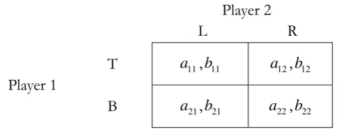
Figure 4 - Asymmetric Coordination Game
In Figure 4, a11a21, a22 a12, b11b12, b22 b21, (a11a21)(b11b12) (a22 a12)(b22b21),
22 11
a a and b22 b11, thus we get that equilibrium (T, L) strictly risk dominates (B, R) while (B, R)
strictly Pareto dominates (T, L). Accordingly, similar to the above examples, the corresponding Pareto optimal endogenous matching reads as follows, i.e.,
( 1, 1), ( 2, 2)
with 1
21 22 22 12 11 21
b b b b b b
and
2
12 22
22 21 11 12
a a a a a a
. Then, (B, R) can be seen as an induced game equilibrium in the present case.
3. Formulation
3.1. Set-up and Assumptions
Let AI1I2 be the payoff matrix for row-players and BI1I2 be the payoff matrix for column-players
with AI1I2, BI1I2 1 2
II
, and I1, I21. Here, and throughout the current paper, we study the
Player 1
T a11,b11 a12,b12
replicator dynamics of I1I2 normal form games between two groups of populations. Put
1 1
1 1 ( ) ( )
I i
i M t M t
, where Mi1( )t denotes the number ofstrategy-1
i players at period t. Similarly, let 2 2
2 1
( ) ( )
I i
i N t N t
, where Ni2( )t denotes the number ofstrategy-2
i players at period t.
We let Xi1( )t Mi1( )t M t( ), Yi2( )t Ni2( )t N t( ) denote the frequencies of strategies
1
i
and i2, respectively, with i11, 2,...,I1 and i2 1, 2,...,I2. Therefore, the average payoffs of
strategy i1 and strategy i2 are given by u i Y t
1, ( )
1 ( )T i
e AY t and
2, ( )
2 ( )T T i
u i X t e B X t ,
respectively, with the superscript “T” denoting transpose, and X t( )
X t1( ),...,Xi1( ),t ..., 1( )
T I
X t ,
( )
Y t
Y t1( ),...,Yi2( ),t ...,YI2( )t
T, and also1 (0,...,1,..., 0)
T i
e , 2 (0,...,1,..., 0)T
i
e , where the
1
i -th entry and i2-th entry are ones, respectively, for i11, 2,...,I1 and i2 1, 2,...,I2.
Specifically, in the current paper, we employ the following endogenous matching by incorporating two vectors, i.e.,
1,...,i1,...,I1
TI1 and ( ,...,1 i2 ,...,I2)TI2 with1 1
11 0
I i i
and 2 22 1 0
I i i
, into the present model. Now, the generalized average payoffs ofstrategies i1 and i2 are rewritten as u i Y t
1, ( )
1
( )
1 ( ) 1T T T
i i i
e A Y t e AY t e A and
2, ( )
2
( )
T T i
u i X t e B X t
2
T i
e
2
( )
T T T i
B X t e B , respectively, for i11, 2,...,I1 and
2 1, 2,..., 2
i I . In other words, u i Y t
1, ( )
and u i X t
2, ( )
can be seen as 1T i
e A -
perturbation and e BiT2 T-perturbation of u i Y t
1, ( )
and u i X t
2, ( )
, respectively. Moreover, asgreat loss of generality name the two vectors, to be determined, as the endogenous matching is for the sake of convenience and also with the purpose of capturing the essence of the problem facing us. To sum up, we argue that, in the present case and in some sense, what the present state is will not be important, what the goal will be is also not important, the only important matter we care about is what we need to lead us from the present state to our goal. Here, the endogenous matching defined by the two vectors meets our need.
We now denote by
(Wi), (Wi),
( )0 ( )
i i W t t ( )
,Wi
the filtered probability space with
(Wi)
( )0 ( )
i i W t t
the (Wi) augmented filtration generated by d dimensional
standard Brownian motion
Wi( ), 0t t i( )
with (Wi) ( )( ) i i W
, (Wi) and
( )
i
a stopping time, to be endogenously determined. Moreover, we define
,
i i
N dt dz
N1i
dt dz, 1i
,...,
,
T i i n n
N dt dz
1
, 1
1 1 ,...,
,
T i i i i i i i i
n n n n
N dt dz dz dt N dt dz dz dt ,
in which
1 n i l
l
N
are independent Poisson random measures with Lévy measures li
coming
from n independent (1-dimensional) Lévy processes 1 ( ) i
t
0 1 1 1
0 ,
t i i i
z N ds dz
, …, ( ) i n t
0 0 ,t i i i n n n
z N ds dz
with 0
0 , and then the corresponding stochastic basis isgiven by
(Ni), (Ni),
( )0 ( )
i i N t t
,(Ni)
with (Ni)
( )0 ( )
i i N t t
the (Ni)
augmented filtration and (Ni) ( )
( ) i i N
, (Ni) and i( )
a stopping time, to be endogenously determined. Thus, we are provided with a new stochastic basis
i,i,
0 i ( )i t t
,i
, where i (Wi)(Ni)
, i (Wi) (Ni)
, ti
(Wi )
t
(Ni )
t
,
i
(Wi) (Ni)
and i
0 i ( ) i t t
denotes the corresponding filtration satisfying the
well-known “usual conditions”. Here, and throughout the current paper, i
is used to denote the expectation operator with respect to (w. r. t.) the probability law i
for 1, 2. Naturally, we have stochastic basis
,,
0 ( ) t t
,
with iI i
,
I i
i
, t
I i
i t
, iI i
, ( ) iI i ( )
iI i ( )
if 1, and
( )
iI i ( )
iI i ( )
if 2 with ,
0 ( ) t t
denoting the
corresponding filtration satisfying the usual conditions, and is used to denote the expectation operator w. r. t. the probability law for 1, 2. Furthermore, we are led to the following probability space
, ,
0 ( ), t t
with 2 1
, 2 1
, t 2 1 t
,
2 1
, ( ) 2 1 ( )
with ,
t 0 t ( ) denoting the corresponding filtration satisfying the usual conditions, and is used to denote the expectation operator w. r. t. the probability law .We now define the canonical Lebesgue measure on measure space
, B
with
0,
, (0, ) and B
the Borel sigma-algebra, and also the correspondingregular properties about Lebesgue measure are supposed to be fulfilled. Thus, we can define the following product measure spaces
i
, i
B and
,B
withcorresponding product measures i
and , respectively, for i 1, 2,...,I and for 1, 2.
Now, based upon the probability space
i,i, i
,i
for 1, 2, and following Fudenberg and Harris (1992), Cabrales (2000), Imhof (2005), Benaïm et al (2008), Hofbauer and Imhof (2009), the stochastic replicator dynamics26 of the two groups of populations can be
respectively given as follows,
1 1
1 1 1 1 1 1
1 1 1 1 1 1 1 1 1
0
1 1 1 1
( ) ( ) ( ) ( ) ( ) , ,
d n
i i T i i i i
i i k k i l l l l
k l
dM t M t e AY t dt t dW t t z N dt dz
,
2 2
2 2 2 2 2 2
2 2 2 2 2 2 2 2 2
0
2 1 2 1
( ) ( ) ( ) ( ) ( ) , ,
d n
i i T T i i i i
i i k k i l l l l
k l
dN t N t e B X t dt t dW t t z N dt dz
.where Mi1( )t is assumed to be i1
B adapted, Ni2( )t is i2
B adapted, Y t( )
is also assumed to be 2B
adapted, X t( ) is 1B
adapted, i k1 1( )t and
1 1 1 , 1i i l t zl
are i1
B progressively measurable, and
2 2( )
i k t
and
2 2 2 , 2i i l t zl
are i2
B
progressively measurable, for 1 1, 2,..., 1
i I , i2 1, 2,...,I2, k11, 2,...,d1,
2 1, 2,..., 2
k d , l11, 2,...,n1 and l2 1, 2,...,n2. Thus, based upon the above SDEs, we get the following proposition,
PROPOSITION 1: The Lyapunov exponents of the above SDEs are,
11
1 1 1 1
2 1
2 1
0
1 1
lim log i( ) lim t T ( ) d ( )
i k i k
tt M t tt
e AY s
s
1 1 1 1 1
1 1 1 1 1 1 1 1
1 1 0 log 1 , ,
n i i i i
i l l i l l l l l s z s z dz ds
a.s.
And,
22
2 2 2 2
2 1
2 1
0
1 1
lim log i ( ) lim t T T ( ) d ( )
i k i k
tt N t tt
e B X s
s
2 2 2 2 2
2 2 2 2 2 2 2 2
2 1 0 log 1 , ,
n i i i i
i l l i l l l l l s z s z dz ds
a.s.
respectively, for Mi1(0)0
, Ni2(0)0
and i11, 2,...,I1, i2 1, 2,...,I2. Hence, the above SDEs
are almost surely exponentially stable if and only if,
11 1 1 1
2 1
2 1
0
1
lim t T ( ) d ( )
i k i k
tt
e AY s
s
1 1 1 1 1
1 1 1 1 1 1 1 1
1 1 0
log 1 , , 0
n i i i i
i l l i l l l l l s z s z dz ds
.
And,
22 2 2 2
2 1
2 1
0
1
lim t T T ( ) d ( )
i k i k
tt
e B X s
s
2 2 2 2 2
2 2 2 2 2 2 2 2
2 1 0 log 1 , , 0
n i i i i
i l l i l l l l l s z s z dz ds
.
respectively, for i11, 2,...,I1 and i2 1, 2,...,I2.
So, we directly provide the following assumption,
ASSUMPTION 1: Here, and throughout the current paper, we suppose that,
11 1 1 1
2 1
2 1
0
1
lim t T ( ) d ( )
i k i k
tt
e AY s
s
1 1 1 1 1
1 1 1 1 1 1 1 1
1 1 0
log 1 , , 0
n i i i i
i l l i l l l l l s z s z dz ds
.
And,
22 2 2 2
2 1
2 1
0
1
lim t T T ( ) d ( )
i k i k
tt
e B X s
s
2 2 2 2 2
2 2 2 2 2 2 2 2
2 1 0 log 1 , , 0
n i i i i
i l l i l l l l l s z s z dz ds
.
always hold.
Now, based upon Proposition 1 and Assumption 1, we, without loss of generality, introduce the following technical assumption,
ASSUMPTION 2: Throughout the current paper, both M t( ) and N t( ), sufficiently large, are assumed to be finite constants.
REMARK 3.1: Some of existing literatures (see, Nowak et al., 2004; Imhof and Nowak, 2006, and among others) have confirmed that Assumption 2 has very important implications. That is to say, on the one hand, Assumption 2 is used to make things much easier from the viewpoint of pure mathematics; and also, Assumption 2 is indeed without loss of any generality in the sense of economic and biological intuitions on the other hand (see, Fudenberg and Levine, 1993; Young, 1993; Binmore et al., 1995; Binmore and Samuelson, 1997).
Notice from Assumption 2 that the sizes of the two populations are finite constants, based on Itô’s rule one can easily find,
1 1
1 1 1 1 1 1
1 1 1 1 1 1 1 1 1
0
1 1 1 1
( ) ( ) ( ) ( ) ( ) , ,
d n
i i T i i i i
i i k k i l l l l
k l
dX t X t e AY t dt t dW t t z N dt dz
1 1 1 1 1 1 1
1 1
0
( ) ( ) ( ) ( ) n , ,
i T i i i i i i
i
X t e AY t dt t dW t t z N dt dz
,
2 2
2 2 2 2 2 2
2 2 2 2 2 2 2 2 2
0
2 1 2 1
( ) ( ) ( ) ( ) ( ) , ,
d n
i i T T i i i i
i i k k i l l l l
k l
dY t Y t e B X t dt t dW t t z N dt dz
2 2 2 2 2 2 2
2 2
0
( ) ( ) ( ) ( ) n , ,
i T T i i i i i i i
Y t e B X t dt t dW t t z N dt dz
, (1)
subject to the initial conditions, i.e., Wi1(0) (0,..., 0) T i1a.s., Wi2(0) (0,..., 0) T i2a.s.,
(0)
2 2
..., i (0),..., I (0) T
Y Y
y1,...,yi2,...,yI2
T y0 2 a.s., Xi1( )t is assumed to be
1
i
B adapted, and Yi2( )t is assumed to be i2
B adapted, for
1
i 1, 2,...,I1
and i2 1, 2,...,I2 . Moreover, with a little abuse of notations, we put
1(0)
i
11(0),
i
1 1
...,i k(0),..., 1 1(0)
T i d
i11, ...,i k1 1,..., 1 1
T i d
i1, i1
0,zi1
111 0, 1
i i z
11 1 1
,..., 0, i ,...,
i l zl
1
1 1 0, 1
T i i n zn
111 1
i i z
11 1 1
,..., i ,...,
i l zl
1
1 1 1
T i i n zn
i1
zi1 , i2(0)
21(0),
i
...,i k2 2(0),...,
2 2(0)
T i d
i21, ...,i k2 2,..., 2 2
T i d
i2 , and i2
0,zi2
2
21 0, 1i i z
,...,
2
2 2 0, 2
i i l zl
,...,
2
2 2 0, 2
T i i n zn
221 1
i i z
,...,
22 2 2
i i l zl
,...,
2
2 2 2
T i i n zn
i2
zi2 , for 1
i 1, 2,...,I1 and i2
1, 2,...,I2. Moreover, we have,
1 1
0
1 1 1 1 1 1 1
( ) ( ) ( ) ( ) I n ( ), ,
dX t f X t dtg X t dW t
h X t z N dt dz ,
2 2
0
2 2 2 2 2 2 2
( ) ( ) ( ) ( ) I n ( ), ,
dY t f Y t dtg Y t dW t
h Y t z N dt dz , (2)
with X t( )
X t1( ),...,Xi1( ),...,t XI1( )t
T and Y t( )
Y t1( ),...,Yi2( ),...,t YI2( )t
T.Next, we are in the position to introduce some necessary assumptions, ASSUMPTION 3: The initial conditions Xi1(0) xi1 0
, Yi2(0) yi2 0
, X(0) x 0 and
(0)
Y y 0 are all supposed to be deterministic and bounded for i11, 2,...,I1 and i2 1, 2,...,I2.
Furthermore, i1 0 i1 a.s., i2 0 i2 a.s.,
1 1 1 , 1i i l t zl
1
1
1 i
l
i1 a.e., and
2 2 2 , 2i i l t zl
2
2
1 i
l
i2
a.e., for 1 1
i l
0 , 2
2
i l
0 and for i1 1, 2, ...,I1 ;
2
i 1, 2,...,I2; l11, 2, ...,n1 and l2 1, 2, ..., n2.
ASSUMPTION 4: The following linear growth and local Lipschitz continuity conditions are fulfilled, respectively,,
1 1
1 1 1
0 1
2
2 2 2
1 1 1 1 1 1 1
2
2 2 1 , 2 1
I n
l l l l
f x g x h x z dz C x
2 2
2 2 2
0 2
2
2 2 2
2 2 2 2 2 2 2
2
2 2 2
1
, 1
I n
l l l l
f y g y h y z dz C y
,
for some constants C1, C2 . And,
2
21 1 1 1
2 2
f x f x g x g x
1 1
1 1
1 1 1 0
1
2 2
1( ) 1 1( ) 1 1 1 1
2 2
1
, ,
I n
l l
l l R l
h x z h x z dz L x x
,
2
22 2 2 2
2 2
f y f y g y g y
2 2
2 2
2
2 2
0 2
2 2
2( ) 2 2( ) 2 2 2 2
2 2
1
, ,
I n
l l
l l R l
h y z h y z dz L y y
,
for any given constants R1, R2 0 with, x 2 x 2 R1, y 2 y 2 R2, and constants 1
1 R
L ,
2
2 R
L that depend only on R1 and R2, respectively, for all x, x I1
and y, y I2
with
1
1( ) 1
,
l
h x z , h1( )l1
x z, 1 representing the1
l -th columns of matrixes h x z1
, 1 , h x z1
, 1 , respectively, and
2
2( ) 2
,
l
h y z , h2( )l2
y z, 2
denoting the l2-th columns of matrixes
2 2
,
h y z , h2
y z, 2
, respectively, forl11, 2, ..., n1 and l21, 2, ...,n2.
REMARK 3.2: (i) Provided Assumption 4, the existence and uniqueness of strong solutions of the Lévy SDEs given in (2) are ensured, respectively.
(ii) Assumption 4 is indeed weak in the following sense, local Lipschitz continuity conditions can be naturally satisfied for any C1 functions or correspondences thanks to the Mean Value Theorem.
(iii) Here, and throughout the current paper, | | is used to denote absolute value, || || 2 is
used to represent both Euclidean vector norm and the Frobenius (or trace) matrix norm, and is used to denote the scalar product.