Thesis by
Shannon Kao
In Partial Fulfillment of the Requirements for the Degree of
Doctor of Philosophy
California Institute of Technology Pasadena, California
2008
c
2008
Acknowledgments
It seems like only a little while ago I arrived in southern California to start graduate studies at Caltech. My six years here have been very rewarding because with great challenge comes great satisfaction. Many of the people here at Caltech and away from campus have contributed to my successes.
As most students do, I must start with my adviser Joe Shepherd. An adviser, or more appropriately a mentor, colors a student’s experience, and my adviser gave me a very well-rounded one. During my tenure, there were shared triumphs and frustrations. He was always available as a sounding board and showed a true interest in being involved with every step of my project. He was stern when appropriate, but also good at giving support and praise when warranted. He instilled a team attitude among our group, and for that reason, I learned about projects other than mine. This has definitely prepared me to attack new topics with gusto.
I also must thank the members of my committees. Dr Pullin and Dr Meiron provided necessary expertise concerning several of the details of my project. Dr Hunt and Dr Colonius graciously agreed, at the last minute, to serve on my candidacy committee. Dr Colonius additionally served on my defense committee. Their outside perspective was essential to assuring that my thesis work is complete and well presented.
Although he was not able to serve on my defense committee, Dave Goodwin has been invaluable. His thermodynamic library, Cantera, made our implementation possible and he provided valuable technical support.
specific problem. Anatoli Tumin, more recently, has been looking at the problem from a different perspective. Discussions with him have illuminated new interesting aspects of the problem to investigate.
Although professors offer years of experience and a big picture view, often peers have been the most helpful with day to day details. Caltech offers a very special environment where students of different disciplines are encouraged to work together, and I have never hesitated to bounce an idea off any of my colleagues. I would like to thank all the members of my group who have been so helpful. Specifically, Dan Lieberman, Florian Pintgen, Jim Karnesky, Sally Moffett, and Philipp Boettcher have been fantastic collaborators and given me a view into the experimental world. Rita Liang, one of our post-docs, was invaluable in the beginnings of my project because she had also worked on this topic.
Possibly the most helpful student was Kazuaki Inaba, another post-doc. We used his software to confirm the predictions from our method. He spent many hours helping me to modify his software to work with our model, and then he graciously ran many of the simulations. Without his input, the confirmation would not have gone as smoothly.
Besides group members, Vaughan Thomas patiently helped me learn to program and work through the mysteries of Cantera; Theresa Kidd, Sharlotte Kramer, and Richard Kramer were wonderful sounding boards; and Mike Rubel provided Linux expertise. In addition to being supportive scientifically, each of these students also made studying at Caltech a memorable experience.
Caltech can be a very one-dimensional place. Thankfully I have had many outlets here in Pasadena to offset the extreme environment. I want to thank Desiree LaVertu, the Glee Club director and my voice teacher. She has been a source of fun and an additional mentor. She hasn’t taught me about science but has kept my view of life more normal. I also want to thank the members of my church choir. Each week, they remind me that there are millions of people in the world who do not do what we do here at Caltech. It is an important reality check and de-stresser.
Abstract
Detonation propagation is unsteady due to the innate instability of the reaction zone structure. Up until the present, investigations of detonation stability have been exclu-sively concerned with model systems using the perfect gas equation of state and primarily single-step irreversible reaction mechanisms.
This study investigates detonation stability characteristics with reversible chemical kinetics models. To allow for more general kinetics models, we generalize the perfect gas, one-step irreversible kinetics, linear stability equations to a set of equations using the ideal gas equation of state and a general reaction scheme. We linearly perturb the reactive Euler equations following the method of Lee and Stewart (1990) and Short and Stewart (1998). Our implementation uses Cantera (Goodwin, 2005) to evaluate all thermodynamic quantities and evaluate generalized analytic derivatives of quantities dependent on the kinetics model.
The computational domain is the reaction zone in the shock-fixed frame such that the left boundary conditions are the perturbed shock jump conditions which we have derived for a general equation of state and implemented for an ideal gas equation of state. At the right boundary, the system must satisfy a radiation condition requiring that all waves travel out of the domain. Unlike the case of a single reversible reaction, in a truly multistep kinetics model, the radiation boundary condition cannot be solved analytically. In this work, we provide a general methodology for satisfying the appropriate boundary condition.
Contents
Acknowledgments iii
Abstract vi
Contents viii
List of Figures xiii
List of Tables xix
Nomenclature xxiii
1 Introduction 1
1.1 Governing Equations . . . 3
1.2 ZND Detonation Model. . . 5
1.2.1 Chapman-Jouguet Detonation Velocity . . . 9
1.2.2 Overdrive Factor . . . 13
1.2.3 Induction Zone . . . 13
1.3 Detonation Instability . . . 14
1.3.1 Experimental Investigations . . . 17
1.3.2 Numerical Investigations of Stability . . . 24
1.4 Kinetics Models . . . 26
2 Base Flow 33
2.1 One-Step Irreversible Perfect Gas Analysis . . . 33
2.2 One-Step Reversible Perfect Gas Analysis . . . 38
2.2.1 Family of Reversible Models with Constant CJ Temperature . . . 41
3 Linear Stability Analysis 43 3.1 Coordinate Transformation . . . 43
3.2 Linear Stability Equations . . . 45
3.3 Left Boundary: Jump Conditions . . . 49
3.4 Right Boundary: Radiation Condition . . . 51
3.5 Shooting Algorithm . . . 55
3.5.1 Newton-Raphson Iteration Scheme . . . 56
3.5.2 Muller’s Method . . . 57
3.6 Output. . . 59
4 Radiation Condition 60 4.1 Frozen Acoustics . . . 61
4.2 One-Step Irreversible Chemistry . . . 63
4.2.1 Traditional Formulation . . . 67
4.3 One-Step Reversible Chemistry . . . 68
4.4 General Formulation — Detailed Chemistry Model . . . 73
5 Linear Stability Results 81 5.1 Base Flow . . . 81
5.2 Unstable Eigenvalues . . . 85
5.2.1 One Dimension . . . 85
5.2.2 Two Dimensions . . . 88
5.2.3 Eigenfunctions . . . 90
5.3 Perturbation Regime . . . 94
5.3.2 Reaction Zone . . . 97
5.4 Neutral Stability . . . 100
5.5 Acoustic Impedance. . . 102
5.6 Tabular Results . . . 104
6 Direct Euler Simulation 114 6.1 Implementation . . . 114
6.2 Confirmation of Linear Stability Results . . . 116
7 Summary 126 7.1 Summary . . . 126
7.2 Future Work . . . 129
7.2.1 Effective Activation Energy . . . 129
7.2.2 Acoustics . . . 129
7.2.2.1 Far from the Reaction Zone . . . 130
7.2.2.2 Reaction Zone . . . 131
Bibliography 133 A Summary of Equations Required for Implementation 144 A.1 Reactive Euler Equations. . . 144
A.1.1 Shock-Fixed Frame . . . 144
A.1.2 Flat-Shock-Fixed Frame . . . 145
A.2 Linear Stability Equations . . . 146
A.3 Left Boundary Condition . . . 147
A.4 Radiation Condition — One-Step Irreversible Chemistry . . . 148
A.5 Required Additional Derivatives . . . 148
A.5.1 One-Step Reversible Model. . . 149
B Transformations 150
B.1 Energy Equation . . . 150
B.2 Flat-Shock-Fixed Frame . . . 151
B.2.1 One-D Transformation . . . 151
B.2.2 Two-D Transformation . . . 153
B.3 Thermicity Equations. . . 154
B.4 Linear Perturbation of the Energy Equation . . . 156
B.5 Linear Perturbation of the Shock Jump Conditions . . . 157
B.6 Decomposition of w . . . 160
B.7 Adiabatic Change Relation . . . 161
C Thermodynamics 163 C.1 Soundspeed . . . 163
C.1.1 Frozen Soundspeed . . . 164
C.1.2 Equilibrium Soundspeed . . . 164
C.2 Enthalpy Derivatives . . . 165
C.3 Derivatives of Temperature. . . 166
C.4 Pseudo-Thermodynamic Function Derivatives — Detailed Chemistry . . 167
C.5 Specific Heat Derivatives — Detailed Chemistry . . . 169
D Chemistry Implementation 171 D.1 Kinetics Models . . . 172
D.2 Net Production Rate Derivatives . . . 176
D.3 Pseudo-Thermodynamic Function . . . 177
D.4 Detailed Kinetics Model . . . 179
D.5 One-Step Irreversible Model . . . 180
D.5.1 Democratic Method. . . 180
D.5.2 Pseudo-Thermodynamic Function Derivative . . . 181
D.6 One-Step Reversible Model . . . 182
D.6.2 Pseudo-Thermodynamic Function Derivatives . . . 186
E Comparison with Previous Studies 187 E.1 One Dimension . . . 187
E.2 Two Dimensions . . . 189
E.3 Analytic Jump Conditions for the Perfect Gas . . . 191
E.4 Comparison of Ideal and Perfect Gas Jump Conditions . . . 193
E.5 Single Progress Variable vs. Two Species Systems . . . 194
E.6 Radiation Condition . . . 197
F Implementing the Analytic Selection Criterion 202 G Example cti File 204 H Method of Characteristics 207 I Wave Hierarchy 209 I.1 Alternate Eigenvector Formulation . . . 209
List of Figures
1.1 ZND structure for stoichiometric hydrogen-air initially at 300 K and 1 atm. (a) temperature and pressure profiles, (b) density and velocity profiles, (c) major species profiles, (d) minor species profiles . . . 7 1.2 Thermicity ( ˙σ) and temperature ZND structure for stoichiometric
hydrogen-air initially at 300 K and 1 atm.. . . 8 1.3 Cartoon depicting the instantaneous shock-fixed frame. . . 9 1.4 Hugoniots (a) Shock wave propagating in a non-exothermic mixture or a
mixture with frozen composition. (b) Shock wave propagating in an exother-mic mixture. . . 11 1.5 Hugoniot and three representative Rayleigh lines illustrating w1 = UCJ as
the minimum wave speed and tangency of Rayleigh line and Hugoniot at the CJ point. . . 11 1.6 Hugoniot, Rayleigh line, and three representative isentropes (equilibrium)
illustrating the tangency conditions at the CJ point. . . 13 1.7 Cartoon defining induction length (∆i,ZN D) and energy release pulse width
(∆e,ZN D) of CJ detonation in stoichiometric hydrogen-air initially at 1 atm
and 300 K. In this case, ∆i,ZN D ≈161 µm and ∆e,ZN D ≈43µm.. . . 14
1.9 Schlieren images of detonation with initial conditions: 2H2-O2-17Ar, P1 = 20 kPa. Detonation is propagating from left to right, and the image size is ≈146 mm. (Reprinted with permission from Austin (2003) Figure 4.2) . . 16 1.10 PLIF image of detonation with initial conditions: 2H2-O2-17Ar, P1 = 20
kPa, T1 = 300 K. Flow direction is left to right, and the image height 75 mm. (Reprinted with permission from Pintgen (2004), Figure 1.4.) . . . . 17 1.11 Sample soot foils with (a) regular cellular structure (initial conditions: 2H2
-O2-17Ar,P1 = 20 kPa) and (b) irregular structure (initial conditions: C3H8 -5O2-9N2, P1 = 20 kPa). Detonation propagated from left to right, and the image height is 152 mm. (Reprinted with permission from Austin (2003), Figure 1.3.) . . . 18 1.12 Soot foil record of the initiation of 2H2-O2-70%Ar mixture. Back wall is to
the left.(Reprinted with permission from Strehlow et al. (1967), Figure 1. Copyright 1967, American Institute of Physics.) . . . 18 1.13 Arrhenius plot of induction time for a range of post-shock states in
stoichio-metric H2-Air initially at standard conditions. The determination of Ea/R
as the slope is shown. . . 19 1.14 Schlieren images of a (a) “weakly unstable” detonation,θ = 5.2 (initial
con-ditions: 2H2-O2-12Ar,P1 = 20 kPa) and a (b) “highly unstable” detonation,
θ = 11.5 (initial conditions: H2-N2O-1.77N2, P1 = 20 kPa). Detonations propagate from left to right, and the field of view is≈146 mm. (Reprinted with permission from Austin (2003), Figure 5.2.) . . . 20 1.15 Schematic representation of the effect of shock strength on focusing for (a)
sound pulses (b) strong shocks. . . 21 1.16 Schematic sketch of near-normal convex and concave shocks and associated
1.17 Single-spin detonation in C2H2-O2-Ar mixture: (a) Open-shutter photo-graph, (b) Constant velocity spin soot foil. (Reprinted with permission from Schott (1965), Figures 1 and 5a. Copyright 1965, Combustion Insti-tute.) . . . 23
2.1 ZND profiles for one-step irreversible mechanism. In this case, ∆i,ZN D/(af1t1/2) = 0.91 and ∆e,ZN D/(af1t1/2) = 0.22. . . 38 2.2 Family of constant TCJ solutions (TCJ = 3599.29 K) for initial conditions
T1 = 300 K, P1 = 1 atm, YA1 = 1, and YB1 = 0. (a) Temperature profiles (b) Thermicity profiles . . . 42
3.1 Cartoons of the two frames of reference discussed in this section: (a) Lab-oratory Frame and (b) Flat-Shock-Fixed Frame. . . 44 3.2 Perturbed shock front in the laboratory frame. . . 50 3.3 Cartoon of the initial domain created for the Newton-Raphson solver by the
initial guesses for the growth rate. . . 56
4.1 Wave decomposition schematic for flow field far from the main reaction zone in systems with reversible kinetics. . . 72 4.2 Roots (c) of (4.3.26) for the first two modes (Lee and Stewart, 1990)
nor-malized by the frozen soundspeedaf. (a) Mode 1 (b) Mode 2 . . . 74
5.1 Comparison of product profiles for varying overdrive and reversibility. Dis-tances indicated are measured from 0.1YBeq to 0.9YBeq. (a)f = 1.2 (b) f = 1.7 82 5.2 ZND structure for two extents of reversibility (a) ∆s/R= 0 (b) ∆s/R=−8
5.3 Unstable eigenvalues for the first four modes (ky = 0). The real part of the
eigenvalue ωI is plotted on the x-axis and the imaginary part ωmathcalR is
plotted on the y-axis. (a) Mode 1 (ky = 0) (b) Mode 2 (ky = 0) (c) Mode
3 (ky = 0) (d) Mode 4 (ky = 0) . . . 86
5.4 Comparison of two-dimensional results from Short and Stewart (1998) (black curves) with results from the current study (red curves). E˜a = ˜β = 50,
γ =f = 1.2, irreversible kinetics. . . 89 5.5 Relative percent difference between digitized data from Short and Stewart
(1998) and data from the current study. E˜a = ˜β = 50, γ = f = 1.2,
irreversible kinetics. Black lines indicate 1% and 10% difference. . . 90 5.6 Schematic of acoustic resonance between the shock front and the energy
release zone.. . . 91 5.7 Unstable modes for three extents of reversibility (∆s/R = 0,−5,−8)
vary-ing transverse wave number ky. Mode 1 (ky = 0): f = 1.2 (solid), f = 1.6
(dashed), Mode 2 (ky = 0): f = 1.2 (solid), f = 1.5 (dashed), and Mode 3
(ky = 0): f = 1.2 (solid) . . . 92
5.8 Eigenfunction profiles z1(x) (3.2.8) for f = 1.2 and (a) Mode 1 (k
y = 0),
∆s/R = 0, (b) Mode 1 (ky = 0), ∆s/R = −8, (c) Mode 2 (ky = 0),
∆s/R = 0, (d) Mode 3 (ky = 0), ∆s/R= 0. . . 93
5.9 −ωτ∗|xR(ae/af) +xR
2 as a function of overdrive for four cases (a) Mode 1 (ky = 0), ∆s/R= 0, (b) Mode 4 (ky = 0), ∆s/R= 0, (c) Mode 1 (ky = 0),
∆s/R =−8, (d) Mode 4 (ky = 0), ∆s/R=−8. . . 96
5.10 Ratio of reaction zone length (τi,ZN D +τe,ZN D/2) to oscillation frequency
(2π/Im(ω)) vs. one-dimensional mode number. Data corresponds to values given in Table 5.4. Linear fit equations are given for each case. (a) ∆s/R = 0,f = 1.2 (b) ∆s/R =−8,f = 1.2 . . . 99 5.11 (a) Neutral stability (Re(ω) = 0) curves for modes one through four with
5.12 Specific complex acoustic impedanceζ = (P0/u0)/(ρaf) forf = 1.2 and (a)
∆s/R = 0 mode 1, (b) ∆s/R = 0 mode 4, (c) ∆s/R = −8 mode 1, (d) ∆s/R =−8 mode 4. A line at ζI = 0 is provided to indicate whereζ is real.103
6.1 Post-shock pressure vs. time for ∆s/R = 0 and (a)f = 1.7088 (b)f = 1.74 generated with Inaba’s software. . . 117 6.2 Discrete Fourier transforms (black) of post-shock pressure vs. time for
∆s/R = 0 and (a) f = 1.7088 (b) f = 1.74 generated with Inaba’s soft-ware. Also shown (red) are discrete Fourier transforms of synthetic histories described by (6.2.1). Spectra are displaced for clarity. . . 119 6.3 Direct Euler Simulation cases superposed as black squares on the neutral
stability curves for modes one and two (see Figure 5.11). Case numbers refer to Table 6.2.. . . 119 6.4 Post-shock pressure histories from direct Euler simulations. (a) Case 1, (b)
Case 2, (c) Case 3, (d) Case 4, (e) Case 5, (f) Case 6 . . . 120 6.5 Post-shock pressure spectra from direct Euler simulations (black) and
syn-thetic spectra using linear stability results (red). (a) Case 1, (b) Case 2, (c) Case 3, (d) Case 4, (e) Case 5, (f) Case 6. Spectra are displaced for clarity. 121 6.6 Post-shock pressure histories from direct Euler simulations. (a) Case 9, (b)
Case 10, (c) Case 11, (d) Case 12, (e) Case 13, (f) Case 14 . . . 123 6.7 Post-shock pressure spectra from direct Euler simulations (black) and
syn-thetic spectra using linear stability results (red). (a) Case 9, (b) Case 10, (c) Case 11, (d) Case 12, (e) Case 13, (f) Case 14. Spectra are displaced for clarity. . . 124 6.8 Post-shock pressure histories from direct Euler simulations. (a) Case 7 (b)
Case 8 . . . 124 6.9 Post-shock pressure spectra from direct Euler simulations (black) and
7.1 Categorization of detonation front structure from stability considerations. Parameters for mixtures considered in this study (symbols) are compared to the neutral stability boundary from Lee and Stewart (1990). Activation energy is calculated using the procedure described in Schultz and Shepherd (2000) from one-dimensional constant volume explosion assumption with detailed kinetics. MCJ is calculated using STANJAN. (Reprinted with
per-mission from Austin (2003), Figure 1.6.) Current study data (Table 2.1) included for reference. . . 130 7.2 Comparison of unstable eigenvalues with uncoupledC(7.2.1) (open squares)
List of Tables
1.1 Partial hydrogen oxidation mechanism and rate constants (Smith et al., 1999). 28
2.1 Reversibility parameters forTCJ = 3599.29 K. . . 42
4.1 Reactions and Arrhenius parameters (1.4.5) for the hydrogen-oxygen mech-anism. Arrhenius parameters from GRI Mech 3.0 (Smith et al., 1999). . . 75 4.2 Chemical time scales far from the main reaction zone for initial conditions:
stoichiometric hydrogen-oxygen at 300 K and 1 atm. . . 76 4.3 Inverse eigenvalues of N (3.4.6) far from the main reaction zone for initial
conditions: stoichiometric hydrogen-air at 300 K and 1 atm. The eigenval-ues are ordered by the real part from most negative to most positive. The eigenvalue that we believe is relevant to the radiation condition is bolded. Frequencies (Im(ω)) 10−10, 10−8, and 10−6 are given here. . . . . 77 4.4 Inverse eigenvalues of N (3.4.6) far from the main reaction zone for initial
conditions: stoichiometric hydrogen-air at 300 K and 1 atm. The eigenval-ues are ordered by the real part from most negative to most positive. The eigenvalue that we believe is relevant to the radiation condition is bolded. Frequencies (Im(ω)) 10−4, 10−2, and 100 are given here. . . 78 4.5 Inverse eigenvalues of N (3.4.6) far from the main reaction zone for initial
4.6 Inverse eigenvalues of N (3.4.6) far from the main reaction zone for initial conditions: stoichiometric hydrogen-air at 300 K and 1 atm. The eigenval-ues are ordered by the real part from most negative to most positive. The eigenvalue that we believe is relevant to the radiation condition is bolded. Frequencies (Im(ω)) 108 and 1010 are given here. . . . . 80
5.1 ∆i,ZN D and ∆e,ZN D normalized by the initial frozen sound speed for all
extents of reversibility and overdrive f = 1.2. . . 84 5.2 ∆i,ZN Dand ∆e,ZN Dnormalized by the initial frozen sound speed for ∆s/R =
0 and ∆s/R =−8 with varying overdrive f. . . 84 5.3 Comparison between data calculated in this study for ∆s/R = 0 and data
reported in Lee and Stewart (1990). . . 87 5.4 Time scale comparisons for varying extents of reversibility. Complex growth
rates for modes one and four are given for the lowest overdrive value (f = 1.2). 94 5.5 Neutral stability (Re(ω) = 0) overdrive values for modes one through four
with varying extents of reversibility. The approximate crossover value for modes 1 and 2 is given. . . 100 5.6 Specific complex acoustic impedance for the cases shown in Figure 5.12 at
the shock, at the thermicity peak, and far from the reaction zone. . . 103 5.7 Unstable growth rates for ∆s/R = 0 with varying overdrive f for the first
four one-dimensional modes (ky = 0). . . 104
5.8 Unstable growth rates for ∆s/R =−1 with varying overdrivef for the first four one-dimensional modes (ky = 0). . . 104
5.9 Unstable growth rates for ∆s/R =−2 with varying overdrivef for the first four one-dimensional modes (ky = 0). . . 105
5.10 Unstable growth rates for ∆s/R =−3 with varying overdrivef for the first four one-dimensional modes (ky = 0). . . 105
5.12 Unstable growth rates for ∆s/R =−5 with varying overdrivef for the first four one-dimensional modes (ky = 0). . . 106
5.13 Unstable growth rates for ∆s/R =−6 with varying overdrivef for the first four one-dimensional modes (ky = 0). . . 107
5.14 Unstable growth rates for ∆s/R =−7 with varying overdrivef for the first four one-dimensional modes (ky = 0). . . 107
5.15 Unstable growth rates for ∆s/R =−8 with varying overdrivef for the first four one-dimensional modes (ky = 0). . . 108
5.16 Unstable growth rates for ∆s/R = 0 and f = 1.2 with varying transverse wave numberky for the first three two-dimensional modes (ky 6= 0). . . 109
5.17 Unstable growth rates for ∆s/R=−5 andf = 1.2 with varying transverse wave numberky for the first three two-dimensional modes (ky 6= 0). . . 110
5.18 Unstable growth rates for ∆s/R=−8 andf = 1.2 with varying transverse wave numberky for the first three two-dimensional modes (ky 6= 0). . . 111
5.19 Unstable growth rates for ∆s/R = 0 with varying transverse wave number
ky for the first two two-dimensional modes (ky 6= 0).. . . 112
5.20 Unstable growth rates for ∆s/R =−5 with varying transverse wave number
ky for the first two two-dimensional modes (ky 6= 0).. . . 112
5.21 Unstable growth rates for ∆s/R =−8 with varying transverse wave number
ky for the first two two-dimensional modes (ky 6= 0).. . . 113
6.1 Frequency values determined by linear stability calculation (LSC) and direct Euler simulation (DES). . . 118 6.2 Direct Euler simulation cases. . . 120 6.3 Direct Euler simulation (DES) results compared with linear stability
calcu-lations (LSC). These cases are only unstable to Mode 1. . . 122 6.4 Direct Euler simulation (DES) results compared with linear stability
6.5 Direct Euler simulation (DES) results compared with linear stability calcu-lations (LSC) for stability transition cases. . . 123
Nomenclature
Calligraphic characters
A generic reactant species, Eq. (1.4.6)
B generic product species, Eq.(1.4.6)
C Eq. (F11)
D Eq. (F12)
E Eq. (F13)
F Eq. (F14)
R universal gas constant, Eq. (1.1.11) J/K/mol
G Eq. (F15)
H(ω) eigenvalue selection criterion, Eq. (3.4.20)
P discrete Fourier transform ofP(t), Eq. (6.2.2) Pa
Greek symbols
αT coefficient of thermal expansion, Eq.(B1.5) 1/K
α simplifying function, Eq.(4.2.12) 1/s
∆ ˙Ω ΩB,Y˙ B −ΩB,Y˙ A, Eq. (F2) 1/s
∆fh◦ specific heat of formation at standard state, Eq. (2.1.5) J/kg
∆e eB−eA, Eq. (4.2.13) J/kg
∆h, ∆Rh heat of reaction, Eq. (D1.15) J/kg
∆s/R reversibility parameter (∆a6), Eq.(2.2.16)
∆Z Z,YB −Z,YA, Eq.(F3) Pa/s
∆e,ZN D exothermic pulse width, Fig.1.7 m
∆i,ZN D induction length, Eq. (1.3.1) m
˙
Ω net rate of production, Eq.(1.1.6) 1/s
˙
ωi net molar rate of production, Eq. (D1.9) mole/m3/s ˙
σ thermicity, Eq.(1.2.11) 1/s
Angle, Eq. (B6.1)
i efficiency, Eq.(D1.4)
η sonic parameter, Eq.(1.2.12)
γ isentropic ratio, Eq.(1.1.13)
λ wave length, Eq.(5.7) m
λkN eigenvalue of N, Eq. (3.4.8) 1/m
λ cell width, Figure 1.8b m
µ chemical potential, Eq.(D1.12) J/kg
νi stoichiometric coefficient, Eq.(D1.1)
φ equivalence ratio, pg 26
ψ shock speed perturbation, Eq. (3.2.6), Eq. (3.1.1) m
ψ1 constant coefficient, Eq.(3.2.6) m
ρ density, Eq.(1.2.4) kg/m3
θ argument ofα, Eq.(F10)
θ reduced effective activation energy, pg 20 ˜
β nondimensional heat release, pg 35
˜
κ nondimensional normal wave number, Eq. (4.2.18)
˜
κ∗ function of nondimensional normal wave number ˜κ, Eq. (4.2.19)
ζ specific acoustic impedance, Eq.(5.19)
Roman characters
[M] concentration of chaperon molecule, Eq. (D1.4) moles/m3
W mean molecular weight, Eq. (1.1.11) g/mol
A pre-exponential, Eq. (1.4.5) varies
A0 modifiedA, Eq.(2.2.16) varies
ae equilibrium soundspeed, Eq. (C1.7) m/s
af frozen soundspeed, Eq.(C1.6) m/s
ak, bk polynomial coefficients, Eq. (3.4.3), Eq. (1.4.1)
cP specific heat capacity at constant pressure, Eq. (B1.6) J/K/kg
cφ phase speed, Eq. (4.3.25) m/s
ckN characteristic speeds of matrix N, Eq.(4.1.3) m/s
e specific energy, Eq. (1.1.7), Eq.(1.1.12) J/kg
Ea effective activation energy, Eq. (1.3.1) J/kg
Ea0 modifiedEa, Eq. (2.2.16) J/kg
f generic function, Eq. (B2.1)
f overdrive, Eq.(1.2.23)
Fk generic wave function, Eq. (4.2.15)
G Gru¨uneisen coefficient, Eq. (B1.4)
gi specific Gibbs free energy, Eq.(D1.13) J/kg
gk transformed function, Eq. (3.4.9), Eq. (3.4.8)
h specific enthalpy, Eq.(1.2.11) 1/s
i √−1, Eq.(3.2.6)
KC concentration based equilibrium constant, Eq.(2.2.11)
kf forward reaction rate coefficient, Eq.(1.4.5) varies
KP pressure based equilibrium constant, Eq. (2.2.13)
kr reverse reaction rate coefficient, Eq.(2.2.10) varies
ky transverse wave number, Eq.(3.2.6) 1/m
M Mach number, Eq.(1.2.10)
NY number of species, Eq. (1.1.4)
P pressure, Eq. (1.1.3) Pa
Psynthetic synthetic pressure history, Eq. (6.2.1)
Pmodek constant coefficient, Eq.(6.2.1)
R species specific gas constant, Eq. (1.1.11) kJ/K/kg
r magnitude of α, Eq.(F9)
r reaction rate, Eq. (E1.2) 1/s
S characteristic surface, Eq. (H3)
s◦ standard state specific entropy, Eq. (2.1.12) J/kg/K
T temperature, Eq. (1.1.9) K
t time, Eq. (1.1.1) s
T◦ standard state temperature, Eq. (2.1.12) K
v specific volume, Eq.(1.1.1) m3/kg
W molecular weight, Eq.(1.1.6) g/mol
X mole fraction, Eq.(D1.4)
x Cartesian coordinate, Eq. (1.2.2)
xR point where radiation condition is evaluated, pg 51
Y mass fraction, Eq. (1.1.4)
y Cartesian coordinate, Eq. (1.2.1)
Z pseudo-thermodynamic function, Eq. (3.2.13) Pa/s
U shock speed, Eq.(1.2.23) m/s
u velocity component in x direction, Eq. (3.1.3) m/s
v velocity component in y direction, Eq. (3.1.4) m/s
w velocity component in x direction in the shock-fixed frame, Eq.(1.2.2) m/s
D unsteady shock velocity, Eq. (3.1.1) m/s
Sub-scripts $ Super-scripts
( )0 perturbation quantity, Eqs. (3.2.1)–(3.2.5)
( )∗ complex conjugate, Eq. (6.2.2)
( )1 eigenfunction, Eq.(3.2.8)
( )L laboratory frame, pg43
( )o base flow quantity, Eqs. (3.2.1), (3.2.3)–(3.2.5)
( )1 pre-shock state, Eq.(1.2.17)
( )2 post-shock state, Eq. (1.2.17)
( )c characteristic scale
( )f fluid dynamic components only, Eq.(E6.1) ( )I inhomogeneous solution, Eq. (E6.11)
( )i species index, Eq.(1.1.4) ( )j free index
( )n normal component, Eq. (B6.4)
( )p reaction index
( ),m derivative wrtm, Eq.(1.2.2)
( )1/2 value when YB=0.5
( )I imaginary component
( )R real component
( )CJ Chapman-Jouguet quantity, Eq.(1.2.23) ( )n×n top left n×n of matrix
( )shock of the shock, Eq. (3.1.1)
( )xR base flow quantity far from the reaction zone, pg 51
ˆ
( ) constant coefficient, Eq.(3.4.15)
Im( ) real component
Re( ) real component
˜
( ) nondimensional quantity
Vectors and Matrices
u velocity vector, Eq.(1.1.2) m/s
ΛN matrix of eigenvalues of N, Eq. (3.4.7)
A x convective derivative, Eq.(3.2.11)
B y convective derivative, Eq.(3.2.11)
C source matrix, Eq.(3.2.12)
F vector of fluxes, Eq. (6.1.2)
I identity matrix, Eq.(3.2.10)
J Jacobian matrix, Eq. (4.4.1), Eq.(3.5.3)
L matrix of left eigenvectors, Eq.(3.4.7)
mk left eigenvector, Eq.(3.4.11)
N matrix summation, Eq.(3.4.6)
nk right eigenvector, Eq.(3.4.3)
S vector of source terms, Eq. (6.1.2)
Y vector of mass fractions, Eq.(1.1.7)
z solution vector, Eq. (3.2.7)
Chapter 1
Introduction
A detonation is a supersonic combustion wave in which a shock wave and a reaction zone are coupled. The leading shock raises the temperature and pressure of a mixture of fuel and oxidizer initiating a coupled thermal branching-chain explosion. After an induction time, exothermic recombination reactions create product species whose expansion acts as a piston propelling the shock wave forward. The interaction between the leading shock and consequent reaction zone is a defining characteristic of self-sustained detonations.
Experiments and numerical simulations of detonation propagation problems are also characterized by unsteady motion due to the intrinsic instability of the reaction zone structure. This instability may arise due to the sensitivity of the reaction rates to tem-perature fluctuations. Arrhenius (1889) proposed that the reaction rate k depends on temperature in the following way
k∝exp
−Ea
RT
. (1.1)
From this, we see that small fluctuations in the leading shock speed which are mani-fested as small changes in temperature lead to large changes in the reaction rate. While this is the most commonly discussed cause for the instability, several other mechanisms have been proposed. Despite the fact that we only observe the nonlinear stages of this instability in experimental studies, we can numerically examine the linear stages.
exclu-sively been concerned with model systems using the perfect gas equation of state and reaction mechanisms consisting of a small number (usually one) of irreversible reactions. Starting from the one-step model used in the pioneering studies of Erpenbeck (1962) and the reformulated numerical approach in Lee and Stewart (1990), Short (1997), and Short and Stewart (1998), researchers have been making steady progress by considering more complex chemical reaction models and equations of state (Short and Quirk, 1997, Liang and Bauwens, 2005,Liang et al.,2007). While these multi-step models are an im-provement on the one-step model, realistic chemical kinetics involves multiple reversible reactions.
1.1
Governing Equations
The equations of inviscid motion of a real fluid are the so-called reactive Euler equations, which are simply the conservation of mass, momentum, energy, and species. In a fixed (inertial) reference frame, these are:
Dv
Dt =v∇·u (1.1.1)
Du
Dt =−v∇P (1.1.2)
De
Dt =−P
Dv
Dt (1.1.3)
DYi
Dt = ˙Ωi i= 1, . . . , NY (1.1.4)
D Dt =
∂
∂t+u·∇. (1.1.5)
The symbols are: v specific volume, u fluid velocity, P pressure, e specific internal energy, Yi mass fraction of species i, and ˙Ωi net production rate of species i. In more traditional chemical notation (Kee et al.,1987) the net production rate can be expressed
˙
Ωi =vWiω˙i (1.1.6)
where ˙ωi is the net molar production rate of species i per unit volume and Wi is the molar mass of species i.
Real gas equations of state take many forms. One popular formulation used in Euler flow simulations is
In nonreactive flow problems, this is adequate to close the problem in terms of the primitive variable set (v,u, P). However, this is not a complete equation of state and additional thermodynamic information may be required. One potential difficulty is that the net production rate expressions are commonly given in terms of the temperature T
˙
Ωi(T, v,Y). (1.1.8)
This requires the construction of a temperature function
T =T(P, v,Y) (1.1.9)
that is thermodynamically consistent with the e(P, v,Y) function. This problem is discussed at some length by McCahan (1992) and solved for some specific cases. A methodology for systematically extending the ideal gas properties to real gases has been developed by the chemical engineering community (Smith et al.,1996) and has also found application to problems of this type, i.e., the CHEMKIN-RG package (Butler, 1989).
Using appropriate thermodynamic identities, we can re-express the energy equation (see Appendix B.1) as
DP
Dt + a2
f
v ∇·u=− G
v
NY
X
i=1
∂e ∂Yi
P,v,Yj6=i
˙
Ωi (1.1.10)
where af is the frozen soundspeed discussed in Appendix C.1. A simple but important case is the ideal gas equation of state:
P v =RT R = R
W W =
NY
X
i=1
Yi
Wi
!−1
(1.1.11)
e= NY
X
i=1
Yiei(T). (1.1.12)
gaseous detonations. The individual species specific energy functions ek are determined from thermochemical data (see the JANNAF compilation,Gurvich et al. 1989), statistical mechanics, and spectroscopic studies of molecular structure.
For an ideal gas, G= γ−1,αT = 1/T, and cP = γR/(γ−1) where
γ(T) = cP
cv
(1.1.13)
is the temperature-dependent ratio of specific heat capacities. The reactive Euler equa-tions in the laboratory frame for an ideal gas are summarized in Appendix A.1.1.
1.2
ZND Detonation Model
The equations that result as a consequence of transforming to the shock-fixed frame and assuming that the flow is one-dimensional and time-independent, i.e., steady
∂ ∂t = 0
∂
∂y = 0, (1.2.1)
are the set of ordinary differential equations that describe the idealized, steady, reaction zone structure first studied by Zel’dovich (1940), von Neumann (1942), and Doering (1943) and now commonly referred to as the ZND model given below.
wv,x=vw,x (1.2.2)
ww,x=−vP,x (1.2.3)
wP,x+ρa2fw,x=−
G v
NY
X
i=1
e,YiΩ˙i (1.2.4)
These equations can also be expressed as
w,x=− 1 1−M2
G a2
f NY
X
i=1
e,YiΩ˙i (1.2.6)
P,x=ρw 1 1−M2
G a2
f NY
X
i=1
e,YiΩ˙i (1.2.7)
ρ,x=
ρ
w 1 1−M2
G a2
f NY
X
i=1
e,YiΩ˙i (1.2.8)
wYi,x= ˙Ωi (1.2.9)
where, the Mach number is
M = w
af
(1.2.10)
Transforming to the shock-fixed reference frame is similar to the coordinate transfor-mation described in Section 3.1 and Appendix B.2. Note that for exothermic reactions, the term P
ke,YkΩk˙ is negative. The solution for CJ detonation (see Section 1.2.1) in an
initially stoichiometric mixture of hydrogen and air at 300 K and 1 atm is depicted in Fig-ure 1.1. This simulation was performed with the Shock and Detonation toolbox (Browne et al., 2007b) with h2air highT.cti, a hydrogen-air mechanism derived from the GRI 3.0 detailed chemical mechanism (Smith et al., 1999), which contains 12 species and 24 reactions. Detailed mechanisms are discussed further in Section 1.4 and AppendixD.4.
We can also express these equations in terms of thermicity,
˙
σ =X k
W Wk
− hk
cPT
˙
Ωk, (1.2.11)
0 0.5 1 1.5 2 14 16 18 20 22 24 26 28 1500 2000 2500 3000 Distance (mm) Te mperature (K) Pressure (atm) 1 1.5 2 2.5 3 3.5 4 4.5 5 200 400 600 800 1000 1200 V elocity (m/s) Density (kg/m 3)
0 0.5 1 1.5 2
Distance (mm) (a) (b) 0 0.05 0.1 0.15 0.2 0.25 H2 O2 H2O
Major Species
0 0.5 1 1.5 2
Distance (mm) 10-8 10-7 10-6 10-5 10-4 10-3 10-2 10-1 10 H O OH Minor Species
0 0.5 1 1.5 2
Distance (mm)
(c) (d)
Figure 1.1: ZND structure for stoichiometric hydrogen-air initially at 300 K and 1 atm. (a) temperature and pressure profiles, (b) density and velocity profiles, (c) major species profiles, (d) minor species profiles
and the sonic parameter,
0 1 2 3 4 5
1500 2000 2500 3000
Thermicity (1/s)
Te
mperature (K)
0 0.5 1 1.5 2
Distance (mm)
x106
Figure 1.2: Thermicity ( ˙σ) and temperature ZND structure for stoichiometric hydrogen-air initially at 300 K and 1 atm.
(1.2.6)–(1.2.9) are
w,x = ˙
σ
η (1.2.13)
P,x =−ρw ˙
σ
η (1.2.14)
ρ,x =−
ρ
w ˙
σ
η (1.2.15)
wYi,x = ˙Ωi. (1.2.16)
A more detailed derivation is presented in Appendix B.3. A solution technique for the ZND equations (1.2.13)–(1.2.16) is discussed in detail in Browne et al.(2005).
1.2.1
Chapman-Jouguet Detonation Velocity
The initial conditions for a ZND calculation are determined from the frozen shock jump conditions in an instantaneous shock-fixed frame which fixes the shock location atx= 0, but focuses on one moment in time.
ρ1w1 =ρ2w2 (1.2.17)
P1+ρ1w21 =P2+ρ2w22 (1.2.18)
h1+
w21
2 =h2+ w22
2 (1.2.19)
This situation is illustrated in Figure 1.3. In this case, we use w to represent the normal
Frozen Shock Cold Reactants
P1, ρ1, T1
Shocked Reactants
P2, ρ2, T2
Y1 Y1
w1 = Ushock - u1 w2 = Ushock - u2
Figure 1.3: Cartoon depicting the instantaneous shock-fixed frame.
velocity component relative to the shock in this frame.
The jump conditions are often transformed so that they can be represented in the
P-v thermodynamic coordinates. The Rayleigh line is a consequence of combining the mass (1.2.17) and momentum (1.2.18) conservation relations
P2 =P1−ρ21w 2
The Rayleigh line must pass through both the initial state 1 and final state 2. If we eliminate the post-shock velocity, energy conservation (1.2.19) can be rewritten as a purely thermodynamic relation known as the Hugoniot or shock adiabat.
h2−h1 = (P2−P1)
(v2+v1)
2 (1.2.21)
or
e2−e1 =
(P2+P1)
2 (v1−v2). (1.2.22)
We can solve either (1.2.21) or (1.2.22) to obtain the locus of all possible downstream states P2(v2) for a fixed upstream state. The result P(v) is referred to as the Hugoniot
curve or simply Hugoniot. For a frozen composition or an equilibrium composition in a non-exothermic mixture like air, Figure 1.4a, the Hugoniot curve passes through the initial state. For an equilibrium composition in an exothermic mixture like hydrogen-air, Figure 1.4b, the chemical energy release displaces the Hugoniot curve from the initial state. The Rayleigh line slope is always negative and dictates that the portion of the Hugoniot curve between the dashed vertical and horizontal lines (Figure1.4b) is nonphys-ical. The nonphysical region divides the Hugoniot into two branches: the upper branch represents supersonic combustion waves or detonations, and the lower branch represents subsonic combustion waves or deflagrations.
The advantage of using the Rayleigh line and Hugoniot formulation is that solutions of the jump conditions for a given shock speed can be graphically interpreted in P-v
diagram as the intersection of the Hugoniot and a particular Rayleigh line.
v
P
1 Shock
v
P
1
detonation
nonphysical
deflagration
(a) (b)
Figure 1.4: Hugoniots (a) Shock wave propagating in a non-exothermic mixture or a mixture with frozen composition. (b) Shock wave propagating in an exothermic mixture.
considered to be physically acceptable. According to Jouguet’s rule (Fickett and Davis, 1979), this solution has two distinct features. First the flow behind the wave is subsonic, i.e., w2 < a2 wherea2 is the sound speed behind the wave (see Appendix C.1). The flow
also satisfies the condition of causality, which is that disturbances behind the wave can catch up to the wave and influence its propagation.
0 0.2 0.4 0.6 0.8 1 1.2 1.4 0
5 10 15 20 25 30
v (m
3/kg)
P (atm)
1 CJ
S
W W1 < UCJ
W1 = UCJ
W1 > UCJ
Figure 1.5: Hugoniot and three representative Rayleigh lines illustrating w1 = UCJ as
As first recognized by Chapman (1899), the geometry (Figure 1.5) of the Hugoniot and Rayleigh line impose restrictions on the possible values of the detonation velocity. Below a minimum wave speed, w1 < UCJ, the Rayleigh line and equilibrium Hugoniot do not intersect and there are no steady solutions. For a wave traveling at the minimum wave speed w1 = UCJ, there is a single intersection with the equilibrium Hugoniot. Above this minimum wave speed w1 >UCJ, the Rayleigh line and equilibrium Hugoniot intersect at two points, usually known as the strong (S) and weak (W) solutions. Based on these observations, Chapman proposed that the measured speed of detonation waves corresponds to that of the minimum wave speed solution, which is unique. This leads to the following definition:
Definition I:The Chapman-Jouguet detonation velocity is the minimum wave speed
for which there exists a solution to the jump conditions from reactants to equilibrium
products traveling at supersonic velocity.
From the geometry (Figure 1.5), it is clear that the minimum wave speed condition occurs when the Rayleigh line is tangent to the Hugoniot. The point of tangency is the solution for the equilibrium downstream state and is referred to as the CJ state, as indicated on Figure 1.5. Jouguet (1905) showed that at the CJ point, the entropy is an extreme value and that as a consequence, the isentrope passing through the CJ point is tangent to the Hugoniot and therefore also tangent to the Rayleigh line, as indicated in Figure 1.6 (see Browne et al., 2007a). We conclude that at the CJ point, the flow in the products is moving at the speed of sound (termed sonic flow) relative to the wave. This leads to the alternative formulation (due to Jouguet) of the definition of the CJ condition.
Definition II:The Chapman-Jouguet detonation velocity occurs when the flow in the
products is sonic relative to the wave. This is equivalent to the tangency of the Rayleigh
0.4 0.5 0.6 0.7 0.8 0.9 1 1.1 8
10 12 14 16 18 20 22 24
26 Hugoniot
CJ point
S1 S2=SCJ S3
Rayleigh line
P (atm)
v (m
3/kg)
Figure 1.6: Hugoniot, Rayleigh line, and three representative isentropes (equilibrium) illustrating the tangency conditions at the CJ point.
1.2.2
Overdrive Factor
As discussed in the previous section, CJ detonations are characterized by a sonic plane at the end of the reaction zone. As indicated in by Figure 1.5, detonations can propagate at speeds greater than UCJ. The overdrive factor,f, defined as
f =
U UCJ
2
=
M MCJ
2
(1.2.23)
is a nondimensional measure of the detonation speed. The necessary downstream bound-ary condition is challenging to determine in the case of a CJ wave (see Section 1.3.2), and for this reason, we will concern ourselves strictly with overdriven detonations. In the programs that accompany this document, the shock speed can be specified three differ-ent ways: f,U, or M. In the case that f is specified, UCJ is determined using methods discussed in Browne et al. (2007a).
1.2.3
Induction Zone
exothermic recombination period (Figure 1.7). The induction length, ∆i,ZN D, is de-termined by the location of maximum thermicity while the energy release pulse width, ∆e,ZN D, is the full-width at half-maximum thermicity locations.
0 0.1 0.2 0.3 0.4
Distance (mm)
01 2 3 4 5
Thermicity (1/s)
x106
1500 2000 2500 3000
Te
mperature (K)
0.5
Δ
iΔ
eFigure 1.7: Cartoon defining induction length (∆i,ZN D) and energy release pulse width (∆e,ZN D) of CJ detonation in stoichiometric hydrogen-air initially at 1 atm and 300 K. In this case, ∆i,ZN D ≈161 µm and ∆e,ZN D ≈43µm.
1.3
Detonation Instability
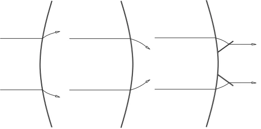
Early experimental investigations of the nonlinear stages of detonation instability pro-vided the historic physical model which relies on the coupling between the fluid mechanics and the chemical reactions. Once the instability is fully developed, in two dimensions, the leading shock speed is a piecewise function of y as shown in Figure1.8a. Classically, the alternating segments are referred to as the slower “incident shock” and faster “Mach stem.” These names are not precise but arise from the shock-wedge interaction problem which was considered analogous. Because the induction length is sensitive to the post-shock temperature which is determined by the post-shock front speed, the distance between the exothermic pulse (see Figure 1.7) and the “Mach stem” is shorter than the distance between the exothermic pulse and the “incident shock.” Figures 1.8and1.9indicate that at each piecewise intersection between segments of “incident shock” and “Mach stem,” a transverse wave propagating perpendicular to the front appears.
t
Mach stem 1
reaction front incident
shock 1 transverse
waves
t2
tracks
t1
incident shock 2 Mach stem 2 shear layer
triple point cell width
flow direction
triple point
λ
(a) (b)
Figure 1.8: (a) Schematic of detonation cellular structure. (Reprinted with permission from Pintgen (2004), Figure 1.3.) (b) Soot foil history of cellular structure (initial con-ditions: 2H2-O2-17Ar, P1 = 20 kPa). (Reprinted with permission from Austin (2003),
Figure 4.2.)
Transverse waves
Lead shock
Triple points Shear layer
(a) (b)
Figure 4.2: Schlieren images of detonation in (a) 2H2-O2-12Ar, P1=20kPa (Shot nc77) (b) 2H2-O2-17Ar,P1=20kPa (Shot nc81). The field of view is about 146 mm. Detonation is propagating from left to right in the narrow channel facility.
4.1.1
Keystones
The induction time is known to be a strong function of the lead shock strength and the
sudden changes in the location of the reaction front are linked to spatial oscillations in
the lead shock which result from the instability of the detonation. As observed in Fig 4.2,
triple points occur at the junction of the transverse wave and lead shock, linking portions
of the lead shock of alternating strength. The local triple point structure is analyzed using
gas dynamics and zero-dimensional chemical species calculations to explain the keystone
features apparent in PLIF images from Pintgen (2000).
Shock and detonation polar calculations (Appendix B) are carried out to analyze
the triple point configurations. This technique has been used previously by several
re-searchers: Oppenheim et al. (1968), Urtiew (1970), Barthel (1972), Subbotin (1975). The
shock polar is calculated using the oblique shock jump relations and assumes a perfect
gas, with the ratio of specific heats taken to be that of the reactants, γ1. The deto-Figure 1.9: Schlieren images of detonation with initial conditions: 2H2-O2-17Ar, P1 = 20
kPa. Detonation is propagating from left to right, and the image size is ≈ 146 mm. (Reprinted with permission from Austin (2003) Figure 4.2)
the segment which was originally traveling faster has decayed significantly (“Mach stem 1” becomes “incident shock 2”), and the portion of the segment that was originally moving more slowly has accelerated (“incident shock 1” becomes “Mach stem 2”). After collision, the transverse waves begin to propagate away from each other, and the cycle begins again. Simulations based on simplified mechanisms and estimates from laboratory experiments suggest that a typical range for shock front velocities is 0.8UCJ to 1.4UCJ.
incident wave
transverse waves
shear layers
triple point tracks Mach stem
Mach stem
a)
b)
c)
Figure 1.4: PLIF image of detonation (
Pintgen et al.
,
2003b
). Flow direction is left
to right. Image height 75 mm. Mixture: 2H
2+O
2+17Ar,
P
0=20 kPa,
T
0=300 K. (a)
and (b) are separate experiments. c) Explanation of features seen in (b).
of the OH radical, an intermediate species in the combustion process (Fig.
1.4
). In
detonations, the OH radical functions as a natural marker for chemical reactions
tak-ing place. Higher fluorescence intensity on the PLIF images corresponds to higher
OH concentration. The PLIF technique allows the selective visualization of certain
species concentrations in a thin layer (corresponding to the light sheet plane) within
the flow field and is discussed in more detail in Chapter
3
. Behind the Mach stem,
a keystone of higher fluorescence is observed. The keystones sometimes appear to be
bounded on the sides by the shear layer. The shear layer is the dividing line between
particles which have passed through the incident shock and transverse wave, and the
particles which have passed through the Mach stem (Fig.
1.3
a). The details in the
corner of the keystone were observed to depend on the mixture type (
Pintgen et al.
,
2003a
).
Note that the cellular structure is three-dimensional and the triple-points shown
in the two-dimensional view shown in Fig.
1.3
a are actually triple lines which extend
into the paper plane. Furthermore, a second set of transverse waves traveling in the
direction perpendicular to the paper plane exists. The triple lines do not necessarily
form an orthogonal grid but may have a random phase and orientation. For
deto-nations with a regular cellular structure propagating in a rectangular cross section
channel, the transverse waves are more likely to be aligned parallel to the channel
Figure 1.10: PLIF image of detonation with initial conditions: 2H2-O2-17Ar, P1 = 20
kPa, T1 = 300 K. Flow direction is left to right, and the image height 75 mm. (Reprinted
with permission from Pintgen (2004), Figure 1.4.)
1.3.1
Experimental Investigations
Clearly, detonations have a somewhat periodic instability which varies with chemical mixture. This prompted researchers to investigate the character of the instability and the important parameters governing the behavior. Shown in Figure 1.11 are two soot foils; Figure 1.11a depicts a “regular” cellular structure and Figure1.11b depicts a very “irregular” structure. “Regularity” is a subjective classification related to the consistency of the cell size and shape. The cell widthλ, defined in Figure1.8, is a characteristic length scale which is usually an average of several cell widths. If all cells are relatively the same size, the mixture is deemed “regular,” but if many different cell sizes and shapes are apparent, the mixture is deemed “irregular.” The appearance of soot foils was used by both Strehlow and Biller (1969) and Libouton et al. (1981) to subjectively characterize detonation stability.
(a) (b)
Figure 1.3: Sample soot foils with (a) regular cellular structure in 2H2-O2-17Ar, P1=20 kPa (Shot nc38) and (b) irregular structure in C3H8-5O2-9N2,P1=20 kPa (Shot nc47). Detonation propagated from left to right and foils were mounted downstream of the window section of the narrow channel. Image height is 152 mm.
with more than 60% argon dilution were found to have excellent regularity. There was no
apparent effect in H2-O2with up to 50% N2dilution. The addition of CO2was also found not to improve the regularity. C2H4-3O2soot foils were reported to be considerably more complex than hydrogen-oxygen foils. The regularity of CH4-2O2and C3H8-5O2 mixtures was classified as poor. These classifications are based on rather subjective observations
and serve only to define broad categories.
A more quantitative analysis of regularity was made by Shepherd et al. (1986) who
used peaks in the power spectral density computed from digital images of soot foils to
identify the frequencies present. Their results confirm the classification described by
Strehlow (1969) for hydrogen and acetylene with argon and nitrogen dilution. Regularity
of cellular structure has been linked to the activation energy of the mixture (Ul’yanitskii,
1981) and mixtures with higher activation energy generally have a more irregular
struc-ture. However, Shepherd et al. (1986) found that this parameter does not fully account
for the observed variations in a systematic way.
1.2.2
Detonation structure and propagation
Although classification of detonation structure by regularity is not rigorous, it has been
useful in the sense that there is evidence of differences in structure and propagation
mech-anism in detonation fronts with different chemical composition which loosely correspond
(a) (b)
Figure 1.3: Sample soot foils with (a) regular cellular structure in 2H2-O2-17Ar,
P1=20 kPa (Shot nc38) and (b) irregular structure in C3H8-5O2-9N2, P1=20 kPa (Shot nc47). Detonation propagated from left to right and foils were mounted downstream of the window section of the narrow channel. Image height is 152 mm.
with more than 60% argon dilution were found to have excellent regularity. There was no
apparent effect in H2-O2with up to 50% N2dilution. The addition of CO2was also found not to improve the regularity. C2H4-3O2soot foils were reported to be considerably more complex than hydrogen-oxygen foils. The regularity of CH4-2O2and C3H8-5O2 mixtures was classified as poor. These classifications are based on rather subjective observations
and serve only to define broad categories.
A more quantitative analysis of regularity was made by Shepherd et al. (1986) who
used peaks in the power spectral density computed from digital images of soot foils to
identify the frequencies present. Their results confirm the classification described by
Strehlow (1969) for hydrogen and acetylene with argon and nitrogen dilution. Regularity
of cellular structure has been linked to the activation energy of the mixture (Ul’yanitskii,
1981) and mixtures with higher activation energy generally have a more irregular
struc-ture. However, Shepherd et al. (1986) found that this parameter does not fully account
for the observed variations in a systematic way.
1.2.2
Detonation structure and propagation
Although classification of detonation structure by regularity is not rigorous, it has been
useful in the sense that there is evidence of differences in structure and propagation
mech-anism in detonation fronts with different chemical composition which loosely correspond
(a) (b)
Figure 1.11: Sample soot foils with (a) regular cellular structure (initial conditions: 2H2
-O2-17Ar, P1 = 20 kPa) and (b) irregular structure (initial conditions: C3H8-5O2-9N2,
P1 = 20 kPa). Detonation propagated from left to right, and the image height is 152
mm. (Reprinted with permission from Austin (2003), Figure 1.3.)
appear spontaneously on a shock which is simply followed by an exothermic reaction,” and that “the transverse waves appear with a regular spacing which has no relation to the tube’s geometry.”
Figure 1.12: Soot foil record of the initiation of 2H2-O2-70%Ar mixture. Back wall is
to the left.(Reprinted with permission from Strehlow et al. (1967), Figure 1. Copyright 1967, American Institute of Physics.)
be obtained from an Arrhenius plot (ln (∆i,ZN D) vs. 1/T). For a one-step model or an elementary reaction with a single activation energy,
ln (∆i,ZN D) =
Ea
R
1
T + constant. (1.3.1)
For a multi-step model, Ea/R can be defined as the local slope of the Arrhenius curve as depicted in Figure 1.13. Schultz and Shepherd(2000) and Pintgen and Shepherd (2003) discuss methods for determining the effective activation energy for multi-step kinetics.
0.4 0.6 0.8 1
10-6
10-5
10-4
10-3
10-2
10-1
100
1000/T
sΔ
iU/UCJ increasing
U/UCJ=1
Experimental Range
Figure 1.13: Arrhenius plot of induction time for a range of post-shock states in stoichio-metric H2-Air initially at standard conditions. The determination of Ea/R as the slope is shown.
The larger the activation energy, the more sensitive the induction length will be to fluctuations in temperature within the reaction zone. Ul’yanitskii (1981) proposed that the effective activation energy is the parameter that governs detonation stability. Radulescu et al. (2002) specifically investigated how argon dilution influences stability. They showed that argon dilution which changes the value of the effective activation energy has a stabilizing affect on C2H2-O2 detonations. Further stability computations
and experimental studies of detonation structure (Austin et al.,2005) have shown that the reduced effective activation energy, θ =Ea/(RT2), is indeed a figure of merit for judging
stability, supporting Ul’yanitskii’s proposal. The larger the value of θ, the more irregular the cellular structure. This is shown in Figure1.14. Although the global activation energy plays a role in detonation stability, Shepherd(1986) showed that activation energy is not a “systematic” measure of regularity.
64
Transverse waves
Lead shock
Triple points Shear layer
(a) (b)
Figure 4.2: Schlieren images of detonation in (a) 2H2-O2-12Ar, P1=20kPa (Shot nc77) (b) 2H2-O2-17Ar,P1=20kPa (Shot nc81). The field of view is about 146 mm. Detonation is propagating from left to right in the narrow channel facility.
4.1.1
Keystones
The induction time is known to be a strong function of the lead shock strength and the sudden changes in the location of the reaction front are linked to spatial oscillations in the lead shock which result from the instability of the detonation. As observed in Fig 4.2, triple points occur at the junction of the transverse wave and lead shock, linking portions of the lead shock of alternating strength. The local triple point structure is analyzed using gas dynamics and zero-dimensional chemical species calculations to explain the keystone features apparent in PLIF images from Pintgen (2000).
Shock and detonation polar calculations (Appendix B) are carried out to analyze the triple point configurations. This technique has been used previously by several re-searchers: Oppenheim et al. (1968), Urtiew (1970), Barthel (1972), Subbotin (1975). The shock polar is calculated using the oblique shock jump relations and assumes a perfect gas, with the ratio of specific heats taken to be that of the reactants, γ1. The
deto-(a) (b)
(c) (d)
Figure 5.2: Schlieren images of weakly unstable detonation: (a) 2H2-O2-12Ar (Shot nc77)
and in (b) 2H2-O2-17Ar (Shot nc81) and highly unstable detonation: (c) H2-N2O-1.77N2 (Shot nc85) and in (d) C2H4-3O2-9N2 (Shot nc148), P1=20 kPa. Field of view is about
146 mm. Detonations propagate from left to right in the narrow channel facility.
(a) (b)
Figure 1.14: Schlieren images of a (a) “weakly unstable” detonation, θ = 5.2 (initial conditions: 2H2-O2-12Ar, P1 = 20 kPa) and a (b) “highly unstable” detonation,θ = 11.5
(initial conditions: H2-N2O-1.77N2, P1 = 20 kPa). Detonations propagate from left to
right, and the field of view is≈146 mm. (Reprinted with permission fromAustin(2003), Figure 5.2.)
with the steady detonation model and then introduces an acoustic source directly be-hind the leading shock. From these initial conditions, he observes the evolution of the wave front emanating from the acoustic source and determines that there is a specific location within the reaction zone where the wave front propagates parallel to the leading shock. Analyzing further, he concludes that high-frequency transverse waves cause all one-dimensional detonations to become unstable.
Barthel and Strehlow (1966) expand on this acoustic theory to describe the finite amplitude structure observed in experiments. They numerically integrated the ray equa-tions for initial condiequa-tions corresponding to Strehlow’s second model. From this, they found that the number of times the wave front contacts the shock front increases with time. Their ray tracing plots indicate that the gradients in soundspeed and flow ve-locity through the reaction zone causes folding in the ray emanating from the acoustic source (Barthel and Strehlow, 1966, see Figure 8).
Sturtevant and Kulkarny (1976) give an in depth discussion of how “wave folding” shown in Figure 1.15a arises for non-reacting acoustic waves. In their experiments, they observe that as the wave speed increases, the wave front no longer folds and instead “Mach reflexion” shown in Figure 1.15b occurs. This is a possible explanation for how the piecewise leading shock develops in detonations.
(a) (b)
Figure 1.15: Schematic representation of the effect of shock strength on focusing for (a) sound pulses (b) strong shocks.
in-vestigated streamline curvature as a function of chemical reaction and found that for sufficiently exothermic reactions, no Crocco point exists. The Crocco point is the zero in the plot of streamline curvature vs. shock angle. At this point, the streamline curvature is zero for all values of the shock curvature. He concludes that in exothermic systems, transverse waves must occur as shown in Figure 1.16. 15
Fig. 4. Streamline to shock curvature ratio in reacting flow forγ = 1.4,
M = 6 andθ= 0.8. The values of the reaction rate parameter are 1/ε =
160 (lowest curve), 80, 40, 20, 0.1, -20, -40, -80, -119, -160, -320
Fig. 5. Schematic sketch of a convex and concave near–normal shocks with associated streamlines, for a perfect gas. Both the concave and the convex shocks produce streamline curvatures that can exist stably in steady flow
4.3 Application to geometrically perturbed normal shock
The fact that the curvature ratio is positive near the normal– shock point, if the rate of an exothermic reaction is suffi-ciently fast, has interesting consequences. In order to under-stand this, consider first the case of a sinusoidally perturbed normal shock in a perfect gas. Figures 2 and 3 show that, for small negative perturbations of the shock angle from
90?, the streamline–to–shock curvature ratio is negative for
a perfect gas. Similarly, for positive perturbations ofβ from
90?, the ratio will be positive. Consequently, a concave–
[image:52.612.187.456.204.337.2]upstream shock, which is associated with streamline conver-gence toward the symmetry plane of the shock, will cause the streamline curvature to be such that streamlines merge into the direction of the symmetry plane, see Fig. 5, left. A convex–upstream shock, for which the deflection is away from the symmetry plane, produces streamlines that bend away from the symmetry plane, see Fig. 5, right. This is very different in the case of a sufficiently fast exothermic reac-tion, of the type where no Crocco point exists, or where the streamline–to–shock curvature ratio is positive in the range 0 < β < 90?. In that case, the situation is as illustrated in Fig. 6. The convex–upstream shock with deflection away from the symmetry plane is also associated with a streamline curvature away from the symmetry plane, see Fig. 6, left. On the other hand, the concave–upstream shock, with deflections
Fig. 6. Schematic sketch of a convex and concave near–normal shocks with associated streamlines, for a gas with fast exothermic reaction rate. The convex–upstream shock on the left can exist with stable steady flow. However, the concave–upstream shock shown in the center requires a pair of unsteady shocks to deflect the flow parallel to the symmetry plane (right)
toward the symmetry plane, also produces a streamline cur-vature toward the symmetry plane. On the symmetry plane, this causes a clash between the two convergent streamlines that will necessarily result in the production of two unsteady shock waves traveling outward from the symmetry plane, see Fig. 6, right.
Thus, it is evident that a concave–upstream shock can not give a steady solution if an exothermic reaction of suffi-ciently fast rate occurs at the shock. This is clearly related to the unsteady waves that occur in detonations and that form the cellular structure observed in such waves.
5 Shock and streamline in the V δ–plane
Many gasdynamical problems are simplified by mapping
the flow into the hodograph oruv–plane. It is sometimes
more convenient to choose other variables for this mapping,
such as theV δ–plane, or thepδ–plane. The condition after a
straight shock in non–reacting flow maps into theV δshock
locus shown in Fig. 7 as the continuous curve, starting at the infinitesimally weak shock point (1,0), moving smoothly
through the maximum–deflection point and back toδ = 0
at the normal–shock point. This curve is the same for flows with finite reaction rate, of course, since it just represents the shock–jump conditions, which we have taken to be the same, by choosing the composition to be unchanged across the shock.
The additional information that is brought into this pic-ture by knowing the gradients at the shock, is that it permits curved and reacting shocks to be treated in this way as well. It is therefore convenient to treat perfect–gas and reacting flows separately.
In particular, the derivativedδ/dV may be formed by
using the general results for the gradients at the shock. Thus, dδ dV = dδ ds ds dV = dδ ds ds dt dt dV = dδ ds(−ρV
2)dt
dp. (45) Substituting from Eqs. (29) and (31), this gives
dδ dV = −
u V v
n
i=2hci dcdti + k
v ρhρG − vV2
ρu px
k F n
i=2hci dcdti + kG ρhρ
v
(46)
This derivative indicates the direction in which the
stream-line departs from the shock in theV δ–plane.
Figure 1.16: Schematic sketch of near-normal convex and concave shocks and associated streamlines for a mixture with fast exothermic reaction rate. The convex upstream shock on the left can exist with stable steady flow. The concave upstream shock shown in the center requires a pair of unsteady shocks to deflect the flow parallel to the symmetry plane shown on the far right.
McVey and Toong (1971) and Alpert and Toong (1972) offer yet another physical argument for the instability. Their proposal, like Strehlow’s second model, argues that acoustic perturbations lead to temperature fluctuations. As described above, small tem-perature fluctuations lead to large changes in the induction length and this affects the leading shock. This model is called the “McVey-Toong short-period wave-interaction model.”
(a)
(b)
Figure 1.17: Single-spin detonation in C2H2-O2-Ar mixture: (a) Open-shutter
photo-graph, (b) Constant velocity spin soot foil. (Reprinted with permission from Schott (1965), Figures 1 and 5a. Copyright 1965, Combustion Institute.)
(1956), and Fay (1952) each developed a theory describing the “spin” behavior, but for some time, the “multi-front” detonation and “spin” detonation were considered separate phenomena. In 1959, Gordon et al. questioned:
Is the spinning wave a completely different regime to that of the normal von Neuman experimental detonation, or can the two regimes be superim-posed?...Is it possible that a spinning wave always results when a stable von Neuman structure cannot be set up?
instability starts the “spin” detonation.
1.3.2
Numerical Investigations of Stability
The model presented in Section 1.2 is unstable to small disturbances and in 1962, Er-penbeck first proposed a numerical approach to determine the hydrodynamic stability of “structurally stable” solutions (Wood and Salsburg, 1960). He focused his attention on a single irreversible reaction mechanism with a perfect gas equation of state. Using this simple model, he was able to determine unstable growth rates and corresponding frequen-cies with a combination of Laplace transform and Fourier transform methods. During the course of the decade, Erpenbeck published thirteen papers furthering his investigation of det