Numerical Study of Detonation Instability
for a Two-Step Kinetics Model
K. Mazaheri
, S.A. Hashemi
1and J.H. Lee
2The stability ofCJdetonations has been investigated numerically with a two-step kinetics model.
The reaction model consists of a non-heat release induction step, followed by an exothermic step. Both steps are governed by the Arrhenius kinetics model. The eect of activation energies associated with these steps on the detonation front behavior has been studied. This study was arranged in two stages. At each stage, one of the activation energies was kept constant and the other one was changed. In the steady detonation structure, the activation energies of the rst and second steps (Ea
1 ;Ea
2) control the induction and reaction lengths, respectively. Increasing Ea
1
(for a xedEa
2) increases induction length and destabilizes a detonation, the same behavior as
a one-step model. IncreasingEa
2rst increases reaction length and has a stabilizing eect (i.e.,
the amplitude of oscillation decreases). Further increasing Ea
2 has a destabilizing eect. The
present study shows that the ratio of the reaction length to the induction length characterizes general features of detonation stability.
INTRODUCTION
Detonation waves are composed of a lead shock that initiates chemical reaction in the combustible mixture and the release of chemical energy, which sustains the lead shock. In this paper, only self-sustaining detonations that travel about the CJ velocity are
studied. Detonations that are supported with pistons and whose velocity is greater than the CJ value, are
not considered here. The rst theoretical work about detonation was the CJ theory that was proposed by
Chapman and Jouguet [1]. They assumed that the thickness of a detonation wave is negligible and the wave travels with a constant velocity. This theory predicts the velocity, pressure and other thermody-namic properties that are in very good agreement with experiments.
The steady, one-dimensional structure of a det-onation wave was rst determined independently by Zeldovich, Von-Neumann and Doring [1] and is known as the ZND structure.
In practice, a stable one-dimensional detonation
*. Corresponding Author, Department of Mechanical Engi-neering, Tarbiat Modarres University, Tehran, I.R. Iran.
1. Department of Mechanical Engineering, Tarbiat Modar-res University, Tehran, I.R. Iran.
2. Department of Mechanical Engineering, McGill Univer-sity, Montreal, Canada.
wave is seldom observed. Experimental observations show that self-sustaining detonation waves exhibit a signicant three-dimensional unsteady structure. How-ever, average velocity is always about the CJ value.
According to Strehlow, the unstable structure of det-onation waves was observed rst by Campbell and Woodhead [2]. Two regimes of detonation instability were observed when blunt-body projectiles were red into a reactive atmosphere [3,4]. The rst involved regular periodic oscillations of the ow eld, while the second showed less regular with larger-amplitude oscillations.
The rst formal linear stability study of detona-tion waves was conducted by Erpenbeck [5], who used a Laplace transform approach to study the behavior of small-amplitude disturbances for a plane steady detonation wave. Parameters that were studied by Erpenbeck are heat of combustion, wave number of dis-turbances and the activation energy of the combustion reaction.
Lee and Stewart [6] developed a normal mode approach to the linear stability problem. They em-ployed a two-point numerical boundary value-shooting algorithm to determine the stability characteristics of detonations. Their study provides highly resolved information about linear stability characteristics, neu-tral stability boundaries and growth rates of unstable disturbances.
and Ludford [7], have been handicapped in the physical interpretations of the various modes of instability. Sharpe [8] developed a new normal mode approach and applied it to a detonation with a single one-step reaction. This method was found to be superior to that of previous researchers in the sense that the CJ case
was well posed and the eect of much higher activation energies was considered.
Most work on the stability analysis of detonations, have used a one-step, irreversible reaction with an Arrhenius form of the reaction rate. In the one-step Arrhenius type reaction model, the linear stability analysis indicates that increasing the activation energy destabilizes the detonation.
In parallel with linear stability analyses, there have been numerous studies concerned with the nu-merical simulation of the pulsating detonation insta-bility with Arrhenius one-step reaction kinetics. Uti-lizing characteristic and nite dierence techniques, respectively, Fickett and Wood [9] and Abouseif and Toong [10] were able to reproduce the salient stability features that were predicted by Erpenbeck. Using advanced numerical methods, a signicant improve-ment in the quality and accuracy of numerical simu-lation was obtained by Bourlioux et al. [11]. Those simulations were able to obtain numerical results in close agreement with the theoretical predictions. In a one-dimensional simulation, the detonation instability appears as the oscillatory behavior of the detonation front. By increasing the activation energy of a one-step model, numerical simulation yields a range of linear oscillation to chaotic oscillatory behavior of the shock front. Stable detonation has a uniform behavior of the shock front and travels with a constant CJ velocity.
The structure of a stable detonation obtained from the numerical simulation is identical to the steady ZND structure.
Short and Quirk [12] carried out linear stability analysis and direct numerical simulation of detonation by making use of a three-step chain-branching reaction model. They used the chain-branching crossover tem-perature as a bifurcation parameter. This parameter controls the ratio of the induction length to the length of the reaction zone. By varying this parameter, the mechanisms of regular and irregular modes of instability and, nally, failure mode, were obtained. Ng and Lee [13], who used this three-step model for studying direct initiation of detonations, suggested that the ratio of induction and reaction zone lengths is the main parameter (independent of the rate process), which characterizes the stability of detonation waves.
A two-step reaction model was used by Sharpe [14] to study the linear stability of pathological detonations. In his model, the rst step was exothermic and the second one was endothermic. He concluded that decreasing the value ofEa
1 Ea
2 (the activation
energy of the rst step minus the activation energy of the second step) tends to destabilize pathological detonations.
Previous works indicated the important role of the induction and reaction lengths on instability. However, no attempt has been made to investigate this role systematically. For example, Howe et al. [15] showed that by changing the heat release rate, the induction delay has a destabilizing eect.
In this paper, a two-step reaction model is used. The rst is a non-heat release induction step and the second is an exothermic reaction. In the next section, the model used for this investigation is presented and the modeling assumption behind it is described. Then, the spatial structure of the steady detonation wave admitted by the model is detailed and a description of how this structure changes, as Ea
1 and Ea
2 are
varied, is presented. Furthermore, the numerical tech-niques used to obtain the numerical simulations of the nonlinear evolution of the pulsating, one-dimensional detonations are outlined and the results of this compu-tational study are discussed. Finally, this paper ends with some conclusions that have been drawn from the investigation.
PHYSICAL MODEL
The detonation is initiated using a blast wave. The chemical reaction is modeled by two-step kinetics. The rst step indicates an induction delay where no heat is released and reactant A is converted to an excited
state,A
. When the rst reaction is near completion,
the second step starts. In the second step, A is
converted to B (product of reaction) and the energy
of the reaction is released. These two steps are shown by two reactions:
A!A
; and A
!B: (1)
The rates of reactions progress are given by:
w 1=
d dt
= K 1
exp
Ea 1 R T
; w
2= d
dt
= K 2
exp
Ea 2 R T
; (2)
where w 1 and
w
2 are reaction rates, K
1 and K
2 are
constant of reactions, T is the absolute temperature, R is the specic gas constant and Ea
1 and Ea
2 are
activation energies. and are progress variables
of two reactions. , which represents consumption of
reactants, decreases in the induction step from 1 to zero. (It is not possible to choose= 0, because the
rst step gives innite time to be completed. Instead, the value of (10 5) was chosen as a typical small value
remains constant during the induction step ( = 1)
and decreases in exothermic step from 1 to zero. The governing equations used are the one-dimensional reactive Euler equations:
@U @t
+@F @x
=s; U = 2 6 6 6 6 4 u e 3 7 7 7 7 5 ; F= 2 6 6 6 6 4 u u 2+ p u(e+p) u u 3 7 7 7 7 5
; s= 2 6 6 6 6 4 0 0 0 w 1 w 2 3 7 7 7 7 5 ; (3)
where variables ;u;p and e are density, particle
ve-locity, pressure and total internal energy, respectively. A polytropic equation of state and an ideal thermal equation of state are used,
e= p ( 1) +
u 2
2 +Q; p=R T; (4)
where Q is the heat release per unit mass of the
reactant and is the ratio of the specic heats.
The dependent variables are non-dimensionalized with respect to the post shock steady-state properties of ZND detonation. Thus, the density, pressure and velocity are non-dimensionalized with the post shock density (
s), pressure ( p
s) and sound speed ( C
s),
respectively. The characteristic length scale, L c, is
chosen arbitrarily as the half reaction length of the steady ZND detonation for Ea
1 = 5 and Ea
2 = 28.
The characteristic time scale ist c= L c =C s. Q;Ea 1and Ea
2 are non-dimensionalized with
R To (for briefness, R To will not be shown in the next sections). In all
calculations here,Q=R To= 50 and= 1:2 are used.
STEADY-STATE ZNDSTRUCTURE
For a set of known parameters (e.g., Q;Ea 1
;Ea 2 and ), detonation may be stable or unstable. Stability
of detonation is determined with numerical simulation of unsteady gas-dynamic equations or linear stability calculations. Here, the rst method is chosen.
The steady-state ZND structure of a detonation represents the structure of a stable detonation. The induction and reaction length of this structure are two meaningful length scales, which have been used by many researchers (e.g., [12,13]) to investigate the dierent detonation dynamic phenomena, such as the instability problem.
The steady-state ZND structure of detonation with two-step chemical kinetics can be determined by neglecting unsteady terms in the governing equations
(Equations 2 to 4). The result is a set of linear dierential equations with respect to X, which could
be solved analytically. This solution is denoted in the following by the superscript*.
It is assumed that the steady detonation prop-agates with the CJ velocity to the left along the
path x l = D CJ t l (superscript
l denotes lab frame
reference), wherex
ldenotes position of shock front and D
CJ is the
CJ detonation velocity, which in terms of Qandis:
D = D CJ = 2 4 1+( 2 1) Q + 1+( 2 1) Q 2 1 ! 1=2 3 5 1=2 : (5) Calculations are performed in a steady shock attached coordinate system (X):
X=x l+ D CJ t l : (6)
Pressure, velocity and density (non-dimensionalized with shock conditions) can be shown to satisfy [6]:
p =
a+ (1 a)(1 bq )1=2 ; u = (1 p ) M s +M s ; = M u ; (7) where: M s 2
= ( 1)D CJ
2+ 2
2D CJ 2 ( 1) ; a= M s
2+ 1
(+ 1) ; b= M s 22
( 1)
(1 a) 2(
+ 1)
: (8)
M
s is the Mach number immediately behind the shock.
The chemical energy release, q
, in the steady wave
satises: q = ^ Q ; (9)
where ^Q=Q=R T
sand the second reaction parameter,
, is assumed as an independent parameter in this
step.
Note that the steady-state variables immediately behind the shock (X = 0), satisfy the shock conditions:
= p = 1 ; u = M s ; = 1 ; = 1 : (10)
In the next step, X must be calculated from the
following kinetics relations:
w 1=
d dt
=u (
) d dX
= K 1
exp
1 p
v
; w
2=
d dt
=u (
) d dX
= K 2
exp
2 p
v
;
1= Ea
1 =(R T
s)
;
2= Ea
2 =(R T
s)
: (11)
It is assumed thatK 1=
K
2. These two parameters are
selected such that length scale becomes half reaction length for Ea
1 = 5 and Ea
2 = 28. Scaling procedure
is further explained in Appendix A.
Since the second step starts after completion of the rst step, it follows that:
X = Z
1 u
( )=w
1(
)d+ Z 1
u (
)=w 2(
)d: (12)
Because in the rst step no heat is released, from Equation 7 it is observed that the pressure, velocity and density remain constant at their initial values and only
varies (see Figure 1). Thus, the length of the rst
step could be obtained from the following equation:
X = Z
1 M
s =w
1(
)d= M
sexp(
1) K
1
Z 1
d
= M sexp(
1) K
1
ln(): (13)
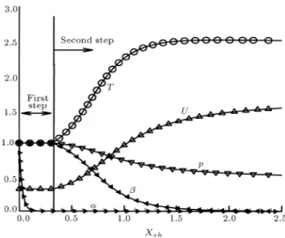
The induction length, from the shock to the location where = 0:95 (in which 5% of the heat of combustion
Figure1. Steady ZND proles for temperature (T),
velocity (U), pressure (p), second reaction parameter ()
and rst reaction parameter () (Q= 50;= 1:2; Ea2= 25 andEa1= 5).
is released) and the reaction length, from the end of the induction length to the location where = 0:05
(in which 95% of the heat of combustion is released), are dened as shown in Figure 2. It is noted that the induction length is the sum of the rst step length to the induction length associated with the second step.
It is interesting to study the changes in the steady wave structure as the activation energies of the two steps,Ea
1 and Ea
2, are varied.
Figure 3 shows the change in the steady wave structure forQ= 50;= 1:2 andEa
2= 20, while the
activation energy of the rst step (Ea
1) varies from 1
to 10. Across the shock, the pressure jumps abruptly to the Von Neumann state. During the induction period, the pressure remains constant. When energy starts to release in the reaction zone, the pressure drops. At the end of the reaction zone, the products are at
Figure 2. Denition of the induction and reaction
lengths in terms of the second reaction parameter ().
Figure 3. Steady ZND proles: Pressure prole for
increasing the activation energy of the rst step (Q= 50; = 1:2 andEa2= 20).
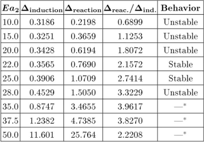
Table1. Values of the induction length (
induction), the
reaction length (reaction) and the ratio of the reaction
length to the induction length (Q= 50;= 1:2 and Ea2= 20).
Ea 1
induction
reaction
reac. =
ind.
Behavior
1.0 0.1651 0.6194 3.7528 Stable 5.0 0.3428 0.6194 1.8072 Unstable 8.0 0.6151 0.6194 1.0071 Unstable 10.0 0.9176 0.6194 0.6751 Unstable equilibrium and the nal state corresponds to theCJ
condition. In Figure 3 it is seen that by increasingEa 1,
the induction length increases. The numerical values of the induction and the reaction lengths for Figure 3 are given in Table 1. It is seen that by increasing
Ea
1, the induction length (induction) increases, while
the reaction length (reaction) remains constant (the
same results were obtained with other denitions of reaction length) and, hence, the ratio of the reaction length to the induction length (reaction
=
induction)
decreases. Since Ea
2 is constant, Ea
1 controls the
induction length.
Figure 4 shows the change in the steady wave structure for Q = 50; = 1:2 and Ea
1 = 5, while
the activation energy of the second step varies. For
Ea
2 = 10, the structure of steady detonation is very
close to the square wave model [6]. For a higher value of Ea
2, the dierence between the structure
of steady detonation wave and this model becomes greater. Table 2 shows the induction and reaction lengths for dierent Ea
2. By increasing Ea
2, the
induction length increases slightly. This is due to increasing the induction length associated with the second step. For Ea
2
> 35, the induction length of
the second step is greater than the induction length of
Figure4. Steady ZND proles: Pressure prole for
increasing the activation energy of the second step (Q= 50;= 1:2 andEa1= 5).
Table2. Values of the induction length (
induction), the
reaction length (reaction) and the ratio of the reaction
length to the induction length (Q= 50;= 1:2 and Ea1= 5).
Ea 2
induction
reaction
reac. =
ind.
Behavior
10.0 0.3186 0.2198 0.6899 Unstable 15.0 0.3251 0.3659 1.1253 Unstable 20.0 0.3428 0.6194 1.8072 Unstable 22.0 0.3565 0.7690 2.1572 Stable 25.0 0.3906 1.0709 2.7414 Stable 28.0 0.4529 1.5050 3.3229 Unstable 35.0 0.8747 3.4655 3.9617 |
37.5 1.2382 4.7385 3.8270 |
50.0 11.601 25.764 2.2208 | * Although this case was not simulated numerically, as noted in the introduction, the instability of this case is obvious.
the rst step, thus,Ea
2controls the induction length.
The reaction length (reaction) increases, when Ea
2
increases. The ratio of reaction length to induction length (reaction
=
induction) increases for Ea
2 < 35
and, then, decreases for Ea 2
> 35. It is seen
that by increasing Ea
2, both induction and reaction
lengths increase. However, for small values of Ea 2
(i.e., Ea 2
< 25), the induction length of the second
step is small relative to the reaction length and the total induction length. Therefore, the induction length approximately remains constant. Above this limit, the induction length of the second step becomes signicant and Ea
2 controls both the induction and reaction
lengths. Decreasing of the ratio (reaction =
induction)
forEa 2
>35 is due to the dominant eect of the second
step. At the limit, when Ea
2 is very large relative
to Ea
1, the two-step model is similar to the one-step
model. Therefore, it can be concluded that small values of Ea
2 control the reaction length and large values
of Ea
2 control both induction and reaction lengths.
Furthermore, this analysis shows the salient features of the two-step model in order to study the individual eects of induction and reaction lengths.
The variation of the ratio of reaction length to the induction length with Ea
2 is drawn in Figure 5.
This ratio has been introduced by many investigators as a criterion, which controls the stability of gaseous detonation, (e.g., [13,15]). For a one-step model, the ratio is decreased by increasing the activation energy. Therefore, for a single-step model, decreasing the ratio causes the instability. Ng et al. [13] obtained the same conclusion for a three-step model. However, the present analysis of the ZND structure for a two-step model predicts that the variation of the ratio with the activation energy of the second step has an extremum (Figure 5). This means that for Ea
2
Figure5. Variation of the ratio of the reaction length to
the induction length vsEa2.
increases with increasing Ea
2 while, for Ea
2 > 35,
the ratio decreases with increasingEa
2. To study the
stability behavior of the two-step model, the complete unsteady gas dynamics equations should be solved. This is the subject of the next section.
NUMERICAL METHOD
Over the past 40 years, a great number of numeri-cal schemes have been devised for the simulation of gas dynamics. In recent years, a number of new shock-capturing schemes, often called high-resolution schemes, have been proposed. Among them are the FCT, MUSCL, ENO and PPM methods. There are several excellent review articles, which compare these schemes from dierent points of view. Interested readers should refer to those articles, particularly the paper of Yang et al. [16] and the Ph.D. thesis of Bourlioux [17]. After comparing dierent schemes, the PPM (Piecewise Parabolic Method) [18] is recom-mended as the best in overall performance. Therefore, in the present work, PPM is chosen as the main gasdy-namics solver. Details of this method are explained in Appendix B.
In analyzing the propagation of pulsating det-onation, the tracking of the shock front plays an essential role. In the past twenty years, several methods have been developed to track the front and other discontinuities in the ow eld. For the purpose of this paper, the simplest one is the conservative front tracking of Chern and Colella [19], which has been utilized in the present study. Since all reactions are completed in a narrow region close to the shock, it is more economical to use a ne grid only in this region and coarse grid elsewhere. To fulll this requirement, a simple version of the \Adaptive Mesh Renement" of Berger and Collela [20] has been used. The entire domain is covered by coarse grids and the ne meshes
are superimposed on the coarse grid near the front. The number of meshes that are necessary, depends on the behavior of the shock front [12]. Unless noted otherwise, the computations were performed using a grid resolution of 20 points in the half-reaction length (L
1=2) as the ne grid. It was observed that further
increases in grid resolution have no eect other than to cause very small changes in the amplitude and period of the shock pressure oscillation. For some cases up to 120 points per half reaction length were used. The developed code is validated via several test problems [21].
RESULTS ANDDISCUSSION
Previous researches have shown that for a one-step Arrhenius kinetics model, the activation energy is the main parameter, which determines the instability of
CJ detonation (e.g., [5,6]). In a one-step model, for a
mixture withQ= 50 and= 1:2, the ZND structure
is unstable for Ea higher than 25 [6]. Increasing the
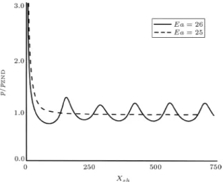
activation energy beyond this limit causes the detona-tion front to exhibit oscillatory behavior as shown in Figure 6. In this gure the shock pressure, normalized with ZND shock pressure, is used for demonstrating detonation front behavior. Therefore, increasingEain
the one-step model destabilizes a detonation.
The eect of the activation energies of the two-step model on detonation front behavior has been studied in this work. Calculations were arranged in two stages. At each stage, one of the activation energies was kept constant and the other was changed. From these results, the front shock pressure is plotted vs the instantaneous shock location.
At the rst stage, the activation energy of the second step was kept constant (i.e., Ea
2 = 20) and Ea
1 was changed. The variation of shock pressure for
Figure 6. Eect of the activation energy of the one-step
Ea
1= 5 is demonstrated in Figure 7. It is seen that the
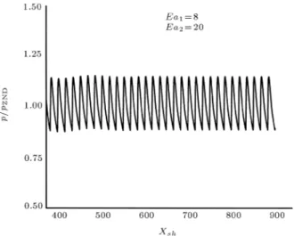
front shows regular oscillation, with small amplitude. Increasing Ea
1 to 8 causes larger amplitude to occur
(Figure 8). An irregular oscillation appears as the activation energy increases to 10 (Figure 9). In this case, it is observed that increasing the activation energy of the induction step promotes detonation instability. This result is similar to that of the one-step model.
Table 1 shows induction and reaction lengths and the stability status of these cases. It is observed that increasing induction length (occurred by increasing
Ea
1) destabilizes detonation. The reaction length
remains constant becauseEa
2 is kept constant. Thus,
decreasing the ratio of reaction length to induction length, as a criterion, causes instability of detonation.
In the second stage of the calculations, the eect ofEa
2on detonation instability has been studied while Ea
1 was kept constant (i.e., Ea
1 = 5). Figure 10
shows the variation of the front shock pressure for
Figure7. Regular oscillation with small amplitude of the
detonation shock pressure forEa 1= 5.
Figure8. Regular oscillation with large amplitude of the
detonation shock pressure forEa1= 8:
Figure9. Irregular oscillation with large amplitude of
the detonation shock pressure forEa1= 10: Ea
2 = 15. An almost regular oscillation with large
amplitude is observed (it is noted that the steady structure of this case is similar to the square wave model, Figure 4). Increasing Ea
2 to 20 causes a
smaller amplitude oscillation with respect toEa 2= 15
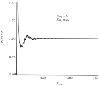
(Figure 11). As Figure 12 shows, further increasing
Ea
2 to 22 stabilizes the front propagation. The front
is also stable forEa
2 = 23 to 25. Figure 13 shows the
detonation front behavior forEa
2= 28. An oscillatory
variation of the front pressure with a very large period (in comparison with other cases) is observed for this case. Therefore, it is concluded that increasing the activation energy of the exothermic step decreases the amplitude of oscillation forEa
2
<22, while increasing
the amplitude forEa 2
>25.
Table 2 shows induction and reaction lengths and the stability status of the above cases. It is observed that by increasing the reaction length and the ratio of the reaction length to the induction length (both occurred by increasing Ea
2), detonation tends to be
Figure10. Regular oscillation with large amplitude of
Figure11. Regular oscillation with small amplitude of
the detonation shock pressure forEa 2= 20.
Figure12. Stable behavior of the detonation shock
pressure forEa 2= 22.
Figure13. Oscillatory variation of the detonation shock
pressure forEa2= 28.
stabilized for Ea 2
< 22. However, for Ea 2
> 25,
detonation becomes more unstable. The behavior of the induction and reaction lengths does not change during increasingEa
2. From Figure 5 it is seen that
by increasing Ea
2, the ratio of reaction length to
induction length increases forEa 2
<35 and decreases
for Ea 2
> 35. As expected, the behavior of this
ratio is changed when detonation is stabilized and then destabilized. However, the change in the behavior of the ratio of the ZND structure does not coincide with the change in the stability status of detonation determined by numerical simulation.
CONCLUSION
Detonation instability (using a two-step chemical ki-netics model) has been studied in this work. It was shown that:
1. For a xedEa
2, increasing Ea
1(i.e., the activation
energy of the induction step) increases the induc-tion length and destabilizes detonainduc-tion, the same behavior as the one-step model;
2. For a xed Ea
1 = 5, increasing Ea
2 (i.e., the
activation energy of the heat release step) increases the reaction length and the induction length. In-creasing the reaction length may have a dominant stabilizing eect forEa
2 <22;
3. For a xed Ea
1 = 5, if Ea
2 increases above 25,
increasing the induction length has a dominant destabilizing eect;
4. The ratio of reaction length to induction length of the ZND detonation characterizes detonation instability, but its behavior does not exactly co-incide with the instability status of detonation, which is determined by the numerical solution of the unsteady governing equations.
REFERENCES
1. Fickett, W. and Davis, W.C., Detonation, University of California Press, CA, USA (1979).
2. Strehlow, R.A., Combustion Fundamentals, McGraw-Hill (1997).
3. Alpert, R.L. and Toong, T.Y. \Periodicity in exother-mic hypersonic ows about blunt projectiles", Acta Astron.,17, pp 538-560 (1972).
4. Kaneshige, M.J. and Shepherd, J.E. \Oblique deto-nation stabilized on a hypervelocity projectile", 26th Symposium (Intern.) on Combustion, The Combustion Institute, p 3015 (1996).
5. Erpenbeck, J.J. \Stability of idealized one-reaction detonations",Phys. Fluids,5, pp 604-614 (1962).
6. Lee, H.I. and Stewart, D.S. \Calculation of linear detonation stability: One dimensional instability of
plane detonation", J. Fluid Mech., 216, pp 103-132
(1990).
7. Buckmaster, J.D. and Ludford, G.S.S. \The eect of structure on the stability of detonations I. Role of the induction zone",Proc. 21th Symp. on Combustion, pp 1669-1675 (1986).
8. Sharpe, G.J. \Linear stability of idealized detona-tions",Proc. R. Soc. Lond.,453, pp 2603-2625 (1997).
9. Fickett, W. and Wood, W.W. \Flow calculation for pulsating one-dimensional detonations",Phys. Fluids,
9, pp 903-916 (1966)
10. Abouseif, G. and Toong, T.Y. \Theory of unstable one-dimensional detonations", Combustion & Flame, 45,
pp 64-94 (1982).
11. Bourlioux, A., Majda, A. and Roytburd, V. \The-oretical and numerical structure for unstable one-dimensional detonations", SIAM J. Appl. Math, 51,
pp 303-343 (1991).
12. Short, M. and Quirk, J.J. \On the nonlinear stability and detonability of a detonation wave for a model three-step chain-branching reaction", J. Fluid Mech.,
339, pp 89-119 (1997).
13. Ng, H.D. and Lee, J.H.S. \Direct initiation of detona-tions with multi-step reaction scheme", Under consid-eration for publication inJournal of Fluid Mechanics
(2001).
14. Sharpe, G.J. \Linear stability of pathological detona-tions",J. Fluid Mech.,401, pp 311-338 (1999).
15. Howe, P., Frey, R. and Melani, G. \Observation concerning transverse waves in solid explosives", Com-bustion Science and Technology,14, pp 63-74 (1976).
16. Yang, H.Q. and Przekwas, A.J. \A comparative study of advanced shock-capturing schemes applied to Burger's equation",J. Comput. Phys.,102, pp 139-159
(1992).
17. Bourlioux, A. \Numerical studies of unstable detona-tions", Ph.D. Thesis, Department of Applied and Com-putational Mathematics, Princeton University, USA (1991).
18. Colella, P. and Woodward, P.R. \The piecewise parabolic method (PPM) for gas-dynamical simula-tions",J. Comput. Phys.,54, pp 174-201 (1984).
19. Chern, I.L. and Colella, P., A Conservative Front Tracking Method for Hyperbolic Conservation Laws, Lawrence Livermore National Laboratory, UCRL 97200 (1987).
20. Berger, M.J. and Colella, P. \Local adaptive mesh renement for shock hydrodynamics", J. Comput. Phys.,82, pp 64-84 (1989).
21. Mazaheri, K. \Mechanism of the onset of detonation in direct initiation", Ph.D. Thesis, Department of Mechanical Engineering, McGill University, Canada (1997).
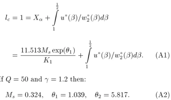
APPENDIXA
Scaling Procedure
The half reaction length of the case (Ea
1 = 5 and Ea
2 = 28) is chosen as length scale. This length can
be calculated from Equation 12.
l c= 1 =
X +
1 2 Z 1
u (
)=w 2(
)d
= 11:513M sexp(
1) K
1
+
1 2 Z 1
u (
)=w 2(
)d: (A1)
IfQ= 50 and= 1:2 then: M
s= 0
:324; 1= 1
:039; 2= 5
:817: (A2)
Calculating Equation A1 givesK 1=
K 2= 33
:45.
APPENDIXB
PiecewiseParabolic Method(PPM)
The Piecewise Parabolic Method (PPM) of Colella and Woodward [18] is a higher-order extension of the Godunov method. To explain PPM, the numerical solution of an initial-boundary value problem is con-sidered for the hyperbolic equation:
u t+
f x= 0
; (B1)
here, u(x;t) is an unknown function of x and t and f(u) is called the ux function. Figure B1 illustrates
space-time domain and indexing.
Equation B1 has the following discretized form:
u n+1
j =
u n j
t
x
(f j+
1 2
f j
1 2)
; (B2)
where x = x j+1=2
x
j 1=2 and t = t
n+1 t
n.
\f" is the ux at the interface between two cells.
Knowing the value of u at time level t
n, the key
to nding the solution at a new time level, t n+1, is
to properly compute the interface uxes, f
j+1=2 and f
j 1=2. Indeed, the dierence between the dierent
methods mentioned above is in the treatment of these uxes.
The main contribution of Godunov is the way in which the uxes are computed. Instead of using some averaging between cell values, in the Godunov method the uxes are computed from an exact solution of the Riemann problem at the interface between two adjacent cells. PPM is a higher-order Godunov method which, instead of using a constant value for the dependent variable at each cell (as in the Godunov method), uses a parabolic prole in each cell with form:
u(x) =u j 1 2 + [u j+ u 6;j(1
)]; (B3)
where: = ( x x j) x ; x j 1 2
xx j+ 1 2 ; (B4) u j= u j+ 1 2 ;L u j 1 2 ;R ; (B5) u 6;j= 6[
u j 1 2( u j+ 1 2 ;L+ u j 1 2 ;R)] : (B6)
The left and right side state variables for the Riemann solver, u
j+1=2;L and u
j+1=2;R, are calculated by rst
using an interpolation scheme to obtainu(x) and then,
an approximation to the value ofuatx
j+1=2, subject to
the constraint thatu
j+1=2 does not fall outside of the
range of values given by u j and
u
j+1. The interface
value is calculated as:
u j+
1 2 = 12(
u j+1+
u j) + 16(
l u j l u j+1) ; (B7) where: l u
j= min ju
j j;2j
j+1=2 j;2j
j 1=2 j sign(u j) ;
if : j+1=2 :
j 1=2
>0; (B8)
l
u j= 0
; otherwise: (B9)
Here,u j = 1 2( u j+1 u j 1)
; j+1=2 = u n j+1 u n j and
j 1=2= u
n j
u n j 1.
In smooth regions away from the high gradients, the left and right states can be computed directly as:
u j+ 1 2 ;L= u j+ 1 2 ;R= u j+ 1 2 ; (B10)
then, the interpolation function is continuous at the interface. If the interpolation function, u(x), takes
on the values, which are not between u
j+1=2;L and u
j+1=2;R, to satisfy the monotonocity condition, more
limitations must be applied. The left and right states,
u
j+1=2;L and u
j+1=2;R, are modied so that
u(x) is a
monotone function on each cell. The new expressions foru
j+1=2;L and u
j+1=2;Rare as follows:
I) u L;j= u R;j = u n j,
if: (u R;j u n j)( u n j u L;j) 0; II) u L;j= 3
u n j 2
u R;j,
if: (u R;j u L;j) u n j 1 2(u R;j+ u L;j) > (u R;j u L;j) 2 6 ; III) u R;j = 3
u n j 2
u L;j,
if: (u R;j u L;j) 2 6 > (u R;j u L;j) u n j 1 2(u R;j+ u L;j) : (B11)
Finally, the cells interface ux is computed as:
f j+
1 2
;L( y) =u
R;j x
2
u
j (1 23 x)u
6;j
;
where:x= y j ; f j+ 1 2 ;R( y) =u
L;j+1 x
2
u
j+1+ (1 23 x)u
6;j+1
;
where:x= y
j+1
: (B12)
In Equations B11 and B12, y = t if > 0 and y= t if<0.
With the left and right states at the interface known, the next step is to solve the Riemann problem to compute the value of the state variables at the interface. Details of the PPM method for the system of Euler equations are described by Colella et al. [18].