Reduced Order Model of Single Machine Infinite Bus Power System Using Stability Equation Method and Self adaptive Bat Algorithm

(1)

Reduced Order Model of Single Machine Infinite Bus

Power System Using Stability Equation Method and

Self-adaptive Bat Algorithm

D. K. Sambariya

∗

,

G. Arvind

Department of Electrical Engineering, Rajasthan Technical University, Kota, 324010, Rajasthan, India

Abstract

In this paper, a largeorder system is reduced by using the self adaptive bat algorithm (SABA) to a reduced-order approximation. The numerator coefficients of a desired reduced-order system are optimized based on integral square error minimization as an objective function pertaining to a unit-step as input. The denominator of the reduced order model is solved by stability equation method. The efficacy of the proposed method is tested with SMIB test systems to get a corresponding reduced-order system. The results are satisfactory in terms of minimum error with the proposed method as compared to Routh approximation and Stability equation based reduced models.

Keywords

Model-order Reduction, Bat Algorithm, Self Adaptive Bat Algorithm (SABA), Stability Equation Method, Integral-square Error Minimization

1 Introduction

High-order system (HOS) is always costly and tedious. MOR is used for simplification of complicated problems in HOS. The selection of the model reduction technique is based on stability equation method as presented in [1]. The pro-cedure of simplification is based on using mathematical ap-proaches. Many methods to solve HOS for reduced order model (ROM) of the system are available in literature [2, 3]. The differentiation method for model order reduction (MOR) of the systems have been proposed in [4, 5, 6]. It follows the simple steps of differentiation of the numerator and denom-inator polynomials but suffers with steady state error in the response of MOR as compared to original system [7, 8]. The methods in literature are not following the stability criterion except the stability equation method [9, 10]. However, mixed method approach is prevalent to consider the stability effect in literature where in numerator and denominator are solved by using different/distinct method as in [11, 12, 13].

Recently, Desai and Prasad have proposed the implemen-tation of order reduction on TMS320C54X processor using genetic algorithm [14]. It also included fourth order exam-ple and reduced to 2nd order model. Pati at el have pro-posed work on sub-optimal control using model order re-duction [15]. Lodhwal and Jha, have proposed the perfor-mance comparison of different type of reduced order mod-eling methods [16, 17]. Model order reduction using stabil-ity equation method [18] and the continued fraction method [19] have been considered for deduction of MOR systems. Sambariya and Prasad have proposed stable reduced model of a Single Machine Infinite Bus (SMIB) Power System with Power System Stabilizer, which is a seventh order system and being reduced to2nd_{order ROM [20, 21, 22, 23].}

MOR is used in industrial applications. The selection of reduction technique is based on the closeness of the reduced order models response to higher order model response [24]. In literature, many authors have considered different methods to solve these problems. The Routh approximation method have been used in [25, 26]. Alsmadi et al have presented the application of Sylvester based model order reduction for a multi-input multi-output (MIMO) power system [27]. It is based on the preservation of stability by retaining dominant poles and minimization of steady-state error. The application of particle swarm optimization (PSO) is examined in [25] by minimizing integral of square error of the response of orig-inal and reduced system. The genetic algorithm (GA) have been considered to determine the free coefficients of numer-ator and denominnumer-ator of discrete transfer function in [28]. Soloklo have presented the application of harmony search algorithm with multi-objective function for determining the lower order model of HO systems [29]. The application of Hermite polynomials with GA is presented for ROM of large systems in [30]. The stable reduced order modeling for lin-ear time invariant systems is presented in [17, 22]. The ap-plication of cuckoo search is considered for deriving reduced order system of HOSs [31].

(2)

or-der linear time invariant systems. The statement of problem is presented in section 2. The stability equation method is de-scribed in section 3. The self-adaptive bat algorithm (SABA) is described in section 4. The system under consideration and the reduced order models are described in section 5. The re-sults on subject of step input signal are discussed in this Sec-tion. Finally the paper is concluded in section 7 and followed by references.

2 Methodology for ROM

Consider a high order transfer function of a system repre-sented as in Eqn. 1.

G(s) =

n∑₋1

i=0 bisi

n

∑

i=0 aisi

(1)

where, theG(s)represents a high order system with the order of n. The purpose of paper is to reduce the order of such high order system to r. The reduced order model may be represented as in Eqn. 2.

R(s) =

r∑−1

j=0 djsj

r

∑

j=0 cjsj

(2)

where,ai,bi,cj anddj are the scalar constants of original

high order system and the reduced order system. The objec-tive is to find a reducedrth _{order system model}_R₍_s₎_such

that it retains the important properties ofG(s)for the same types of inputs.

3 Stability equation method

In this technique, the transfer function of reduced orders are obtained directly from the pole zero patterns of the sta-bility equations of the original transfer function of system [19, 20]. Thus order of the stability equations of transfer function can be reduced [31]. Assuming, a high order trans-fer function the system is as shown in Eqn. 3.

G(s) = bms

m₊_b

m₋1sm−1+....b1s+b0+bo

ansn+an−1sn−1+....a1s+a0

(3)

G(s) =N(s)

D(s) (4)

The Eqn. 4 is the symbolic representation of Eqn. 3. The N(s) andD(s)are the numerator and the denominator of G(s), respectively. The order ofD(s)isnand the order of N(s)is m such that then > m.

3.1

Separation of even,odd parts and reduction

The numerator and the denominator of Eqn. 4 are sepa-rated in even and odd parts. The even and odd polynomials of numerator may be represented by Ne(s)andNo(s),

re-spectively if the even and odd parts are subscribed byeando,

respectively. Similarly, the even and odd polynomials of de-nominator may be represented byDe(s)andDo(s),

respec-tively. Therefore, the system in Eqn. 4 may be represented as following:

G(s) = Ne(s) +No(s)

De(s) +Do(s)

(5)

G(s) =

m

∑

i=0,2,4 bisi+

m

∑

i=1,3,5 bisi

n

∑

i=0,2,4 aisi+

n

∑

i=1,3,5 aisi

(6)

Ne(s) = m

∑

i=0,2,4 bisi

No(s) = m

∑

i=1,3,5 bisi

De(s) = n

∑

i=0,2,4 aisi

Do(s) = n

∑

i=1,3,5 aisi

(7)

The roots ofNe(s)andDe(s)are called zeroszi(s)and

that of No(s) and Do(s) are called poles pi(s). In this

method, a polynomial is reduced by successively discarding the less significant factors. Let us illustrate the method by reducing the denominator, the numerator is reduced similarly and the ratio of reduced numerator and denominator gives the reduced order model. The denominator is separated as following:

D(s) =De(s) +Do(s) (8)

where,

De(s) =a0+a2s2+a4s4+· · · Do(s) =a1+a3s3+a5s5+· · ·

(9) The Eqn. 9 may be written as the following:

De(s) =a0

k1

∏

i=1 (

1 + s2 z2 i )

Do(s) =a1s

k2

∏

i=1 (

1 +s_p22 i

) (10)

wherek1andk2are integer parts ofn/2and(n−2)/2 re-spectively and z12 < p12 < z22 < p22... by discarding the factors with larger magnitude of zi andpi, the reduced

stability equations of desired orderrbecome

Der(s) =ao r1

∏

i=1 (

1 +_zs22 i )

Dor(s) =a1

r2

∏

i=1 (

1 + s_p22 i

) (11)

wherer1andr2are the integer parts ofr/2and(r−1)/2, respectively. The reduced denominator of the system is given as in Eqn. 12.

Dr(s) =Der(s) +Dor(s) (12)

The numerator of the reduced system may be represented as in following Eqn. 13.

(3)

Similarly, the complete model of ther order reduced model may be represented as in Eqn. 14.

R(s) = Ner(s) +Nor(s)

Der(s) +Dor(s)

(14) It may be noted that poles and zeros with smaller magnitude are more dominant than those poles or zeros with larger mag-nitudes. The poles or zeros with larger magnitudes are dis-carded in this technique. Thus the reduced order models pre-serve the dominant performance of the original system.

4 On self-adaptive bat algorithms

The bat algorithm has been introduced by Yang in 2010 [32]. It is based on the behavioral reaction of the microbats to the echolocation based orientation and prey searching. In case of the bat algorithm in [33], the main strategic parame-ters was the loudness and the pulse rate associated to the mi-crobats. The pulse rate regulates an improvement of the best solution while the loudness affects the acceptance of the best solutions. These parameters were kept constant during the iterative search operation of the bat algorithm. The selection of these parameters was a tedious and time-consuming task. In the proposed self-adaptive bat algorithm (SABA), the pa-rameters are adaptive as introduced by Fister in [34]. It serves two purposes (i) initial guess of parameters, (ii) the parame-ter updating, during computational phase. The self-adaptive process enables the control parameters to be changed during the iterative process to select best solutions [35].

The bat algorithm is a population-based algorithm where each microbat represents the candidate solutions. The mi-crobats/candidate solutions may be represented as a vector, pi = (pi1, pi2,· · ·piD)T fori = 1,2,· · ·, Npwith real

val-uedpijin the intervalpij ∈[plb, pub]. Theplbandpub

rep-resents the lower and upper bounds of the particles, andNp

refers to the size to the population of the candidates [36]. The process of the bat algorithm mainly consists of (i) initializa-tion, (ii) variation operainitializa-tion, (iii) local search and evolution of solution, and (v) the replacement [37].

In the initialization process, two main tasks took place such as, (i) parameter initialization of the bat algorithm i.e. set value of pulse rate, loudness and frequency, etc., (ii) ran-dom generation of bat population. The best solution in initial-ization is determined. In variation operator, the virtual bats move according to the rate of echolocation. The current best solution is improved by the random walk in the local search [38, 39].

The behavior of updating is similar to the simulated an-nealing [40], where in the new solutions are selected with the probability of acceptance [41]. In variation operator, the vir-tual bats move towards the best current position according to the following Eqn. 15- Eqn. 17.

fi=fmin+ (fmax−fmin)β (15) v_it=vt_i−1+ (v_it−1−p′)fi (16)

pt_i=pt_i−1+pt_i (17) Theβ represents the random number referring to the Gaus-sian distribution with zero mean and a standard deviation as

unity. The best solution is updated as in Eqn. 18.

pt=best+εAt_iβ (18) The ϵrefers to a scaling factor while theAt

i represents the

loudness of the associatedith_{microbat at instant . The local}

search is started withrias the probability of the pulse rate.

The probability of accepting the new best solutions depends on the loudness Ai. The general phenomena of operation

of the bat algorithm refer to increase in pulse rate, ri and

decrease in loudnessAi, on movement of bat nearer to the

prey [42]. This behavior of microbats can be well defined in terms of following Eqn. 19 - 20.

At_i+1=αAti (19)

r_it=r0_i(1−e(−γε)) (20) Where,αandγare the constants. The parameter controls the rate of convergence of the bat algorithm, andγplays similar behavior as the cooling factor in simulated annealing algo-rithm [39, 43].

It could be easy to say that the bat algorithm in early ap-plications as presented in [38, 40], was the reflection of be-havior of PSO and SA algorithm. The local search bebe-havior refers to PSO behavior, while diversity is associated to SA algorithm in bat algorithm. The exploitation (local search) is associated with the parameter, pulse rate and the exploration to loudness. It means the bat algorithm is able exploitation and exploration during the search process.

The need of self-adaptive behavior of the bat algorithm is to make it free from the initial parameter settings and up-dating of these parameters during the search process [34]. Therefore, the control parameters, pulse rate and loudness are set to self-adaptive to make the self-adaptive bat algo-rithm (SABA). It means the candidate solution represented by pt

i = pti1, pti2,· · ·ptiD needs to be augmented with

in-clusion of pulse rate (rt_{) and loudness (A}t_{). The modified}

representation of candidate solutions may be presented as pt_i = (pt_i₁, pt_i₂,· · ·pt_iD;At, rt)T fori= 1,2,· · · , Np. These

control parameters are modified as by following Eqn. 21 -22.

At+1= {

At_lb+rand0(At_ub−At_lb)if rand1≤τ1

At otherwise

(21) rt+1=

{

rt

lb+rand2(r

t

ub−r

t

lb)if rand3≤τ2

rt _otherwise (22)

The values ofAt_and_rt_{are selected in the range of 0 and 1.}

5 System and reduced order model

5.1

ROM using SE method

Consider a7thorder single-machine infinite-bus (SMIB) power system developed in [17, 21, 23] and presented in Eqn. 23

G7(s) =   2000s

6_{+ 121700}_s5_{+ 1211000}_s4 +7454000s3_{+ 58270000}_s2 +31560000s+ 2075000

  

 s

7_{+ 65}_.₈₅_s6_{+ 984}_.₂_s5_{+ 12130}_s4 +97300s3_{+ 429400}_s2

+2188000s+ 999500

 

(4)

5.1.1 Reduction of numerator

The6th_{order numerator of the system under consideration}

is shown in Eqn. 24.

N6(s) =   

2000s6_{+ 121700}_s5_{+ 1211000}_s4 +7454000s3_{+ 58270000}_s2 +31560000s+ 2075000

(24)

The even and odd parts of the numerator polynomial is separated and presented in Eqn. 25.

N6(s) =

      

2000s6+ 1211000s4+ 58270000s2+ 2075000

| {z }

even

+ 121700s5_{+ 7454000}_s3_{+ 31560000}_s

| {z }

odd

Ne(s) = 2000s6_{+ 1211000}_s4_{+ 58270000}_s2_{+ 2075000} No(s) = 121700s5+ 7454000s3+ 31560000s

(25)

Step-1: Driving the6th_{order to}₄th_{order reduced order of}

numerator polynomial. The reduction process of even pow-ers ofspolynomial in numerator is shown in Eqn. 26. The reduction of even polynomial is shown in Eqn. 26 and the odd polynomial is shown in Eqn. 27.

Ne(s) = 2000s6+ 1211000s4+ 58270000s2+ 2075000

= 1211000s4    1 + 2000

1211000 | {z } 0.001651528 s2

   + 2075000

  

1 +58270000 2075000 | {z }

28.0819277 s2

   

= 1211000s4_{+ 58270000s}2_{+ 2075000}

(26)

No(s) = 121700s5+ 7454000s3+ 31560000s

= 7454000s3

  

1 + 121700 7454000

| {z }

=0.0163268

s2

  

+ 31560000s

= 7454000s3_{+ 31560000}_s

(27)

The 4th _{order reduced order numerator polynomial is}

given in Eqn. 28.

N4(s) = {

1211000s4_{+ 7454000}_s3_{+ 58270000}_s2 +31560000s+ 2075000

(28)

Step-2: Reduction of numerator polynomial from4th_order

to2ndorder polynomial.

N4(s) =

      

1211000s4+ 58270000s2+ 2075000

| {z }

even

+ 7454000_| s3_{z+ 31560000s_} odd =                       

58270000s2

  

1 + 1211000 58270000

| {z }

=0.02078256 s2

  

+ 2075000

+31560000s

  

1 + 7454000 31560000

| {z }

0.23618504 s2     (29)

Step-3: Reduction of numerator polynomial from2nd

or-der to1st_{order polynomial in Eqn. 30.}

N2(s) = 58270000s2+ 31560000s+ 2075000 N1(s) = 2075000 + 31560000s

(30)

5.1.2 Reduction of denominator

The denominator of original system presented in Eqn. 23 is shown in the following Eqn. 31.

D7(s) =   

s7+ 65.85s6+ 984.2s5+ 12130s4

+97300s3+ 429400s2

+2188000s+ 999500

(31)

The even and odd terms of the expression in above Eqn. 31 can be represented as in following Eqn. 32.

Do(s) =s7+ 984.2s5+ 97300s3+ 2188000s

De(s) = 65.85s6+ 12130s4+ 429400s2+ 999500

(32)

Step-1: Reduction of 7th order denominator polynomial to

5thorder as following:

De(s) = 65.85s6_{+ 12130}_s4_{+ 429400}_s2_{+ 999500}

= 12130s4

  

1 + 65.85 12130

| {z }

0.0054286 s2

  

+ 429400s2_{+ 999500}

= 12130s4_{+ 429400}_s2_{+ 999500}

(33)

Do(s) =s7_{+ 984}_.₂_s5_{+ 97300}_s3_{+ 2188000}_s

= 984.2s5

   1 + 1

984.2

| {z }

0.001016 s2

  

+ 97300s3_{+ 2188000}_s

= 984.2s5_{+ 97300}_s3_{+ 2188000}_s

(34)

In this way the reduced5th_{order model of denominator}

poly-nomial can be presented as following in Eqn. 35

D5(s) = {

984.2s5_{+ 97300}_s3_{+ 2188000}_s

+12130s4_{+ 429400}_s2_{+ 999500} (35) Step-2: Reduction of5thorder polynomial to3rdorder poly-nomial.

The odd and even terms of the powers ofsare shown as following in Eqn. 36.

Do(s) = 984.2s5+ 97300s3+ 2188000s

De(s) = 12130s4+ 429400s2+ 999500

(36)

The odd part is reduced by using SE method as in Eqn. 37. Do(s) = 984.2s5+ 97300s3+ 2188000s

= 984.2s5+ 97300s3+ 2188000s

= 97300s3

  

1 + 984.2 97300 | {z } 0.010115

s2

  

+ 2188000s

= 97300s3_{+ 2188000}_s

(37)

The even part is reduced by using SE method as in Eqn. 38. De(s) = 12130s4+ 429400s2+ 999500

= 429400s2

  

1 + 12130 429400 | {z } 0.02824872

s2

  

+ 999500

= 429400s2_{+ 999500}

(5)

The combination of Eqn. 37 and Eqn. 38 gives the3 order reduced denominator polynomial being presented in Eqn. 39. D3(s) = 97300s3+ 429400s2+ 2188000s+ 999500 (39) Step-3: Reduction of3rdmodel to2ndorder Separating the even and odd terms for application of SE method as follow-ing:

D3(s) = 429400s2+ 999500 + 97300s3+ 2188000s

= 429400s2_{+ 999500 + 2188000}_s

  

1 + 97300 2188000

| {z }

0.04446984 s2

   

= 429400s2_{+ 999500 + 2188000}_s

(40)

In this way the2nd _{order reduced denominator polynomial}

can be represented as following in Eqn. 41.

D2(s) = 429400s2+ 2188000s+ 999500 (41) The reduced3rdorder polynomial of the original model us-ing the Eqn. 30 and Eqn. 39 and dividus-ing by 97300 is pre-sented in following Eqn. 42.

R3(s) =

598.8694s2_{+ 324}_.₃₅₇₆_s_{+ 21}_.₃₂₅₇

s3_{+ 4}_.₄₁₃₁_s2_{+ 22}_.₄₈₇₁_s_{+ 10}_.₂₇₂₃ (42) The reduced2nd_{order polynomial of the original model}

us-ing the Eqn. 30 and Eqn. 41 and dividus-ing by 429400 is pre-sented in following Eqn. 43.

R2(s) =

73.4979s+ 4.8323

s2_{+ 5}_.₀₉₅₅_s_{+ 2}_.₃₂₇₇ (43)

5.2

ROM in literature

The reduced model of7th_{order SMIB power system}

de-veloped using Routh approximation method [21] and pre-sented in Eqn. 23 is given as following for ready reference in Eqn. 44.

R2(s) =

81.984s+ 5.390

s2_{+ 5}_.₆₈₄_s_{+ 2}_.₅₉₆ (44)

5.3

ROM using SE and BA

The application of the bat algorithm is used to determine the free elements of the numerator while keeping denomina-tor as found by stability equation method. The problem is considered as optimization with minimization of the integral of square method and defined as in Eqn. 45. TheTsim

rep-resents the settling time. The signal of original system and reduced system are represented byyo andyr, respectively.

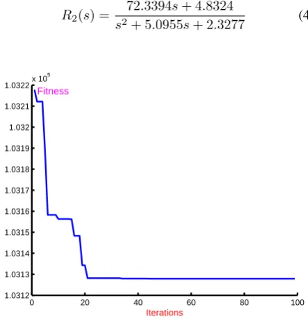
The free elements in numerator areN1andN2and are men-tioned in Fig. 1. The bounds for these parameters are selected as0.01≤N1 ≤100, and0.01≤N2 ≤20. The bat algo-rithm is forced to search optimal values of these parameters within 100 iterations. The fitness function plot during opti-mization in terms of value verses iterations is shown in Fig. 2. The optimal values ofN1 andN2are found as 72.3394 and 4.8324, respectively. Therefore, the2nd order reduced model with bat algorithm and stability equation method can be represented as in Eqn. 46.

errorsignal=

T∫sim

0

|yo(t)−yr(t)|2dt (45)

1 2

2

5.0955 2.3277

N s N

s s

+

+ +

Original system+ +

-Objective Function Bat Algorithm

[image:5.595.319.551.91.240.2]

Step Input

Figure 1. Scheme of determining free coefficients of numerator using bat algorithm

R2(s) =

72.3394s+ 4.8324

s2_{+ 5}_.₀₉₅₅_s_{+ 2}_.₃₂₇₇ (46)

0 20 40 60 80 100

1.0312 1.0313 1.0314 1.0315 1.0316 1.0317 1.0318 1.0319 1.032 1.0321 1.0322x 10

5

Iterations Fmin

Fitness

Figure 2.Plot for fitness function with iterations

6 Results and discussion

[image:5.595.321.543.303.541.2]

(6)

[image:6.595.312.525.104.276.2]

Table 1.Comparison of performance indices of the reduced models

System ITAE IAE ISE

SE-BA-ROM (Proposed) 198.61 109.31 5275.2 Stability Eqn. [23] 198.79 109.41 5275.8 Routh Aprrox. [21] 198.76 109.26 5242.9

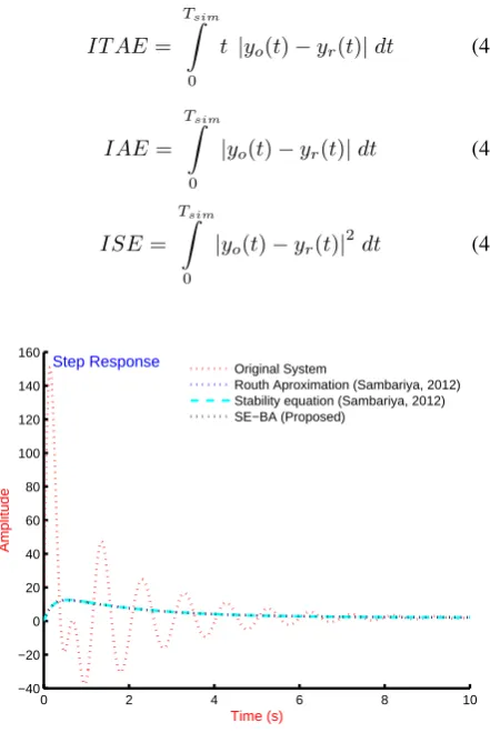
The ITAE value with proposed SE-BA-ROM is 198.61 is comparatively lower in magnitude as compared to that of with SE-MOR [23] and RA-MOR [21] as shown in Table 1. The value of IAE and ISE with proposed SE-BA-ROM are 109.31 and 5275.2, respectively and are lesser as compared to SE-MOR [23] and RA-MOR [21]. It is clear that the re-sponse of the proposed model is with minimum values of per-formance indices; proving its better behaviour as compared to other reduced models. However, it can be observed that the numeral values of performance indices are not having great difference. The overshoot with SE-BA-ROM is reduced as compared to SE-MOR [23] and RA-MOR [21] and is shown in Fig. 4.

IT AE=

T∫sim

0

t |yo(t)−yr(t)|dt (47)

IAE=

T∫sim

0

|yo(t)−yr(t)|dt (48)

ISE=

T∫sim

0

|yo(t)−yr(t)|

2

dt (49)

0 2 4 6 8 10

−40 −20 0 20 40 60 80 100 120 140 160

Time (s)

Amplitude

Step Response _{Original System}

Routh Aproximation (Sambariya, 2012) Stability equation (Sambariya, 2012) SE−BA (Proposed)

Figure 3.Step response of original system and reduced models

7 Conclusion

A bat algorithm based model order reduction is carried out with minimization of ISE pertaining to a unit step input. The optimization process is for bounded constraints resticted to numerator free coefficients while the denominator is solved by stability equation method. The performance of the SE-BA-ROM is compared to Routh approximation method and

0 1 2 3 4 5

0 2 4 6 8 10 12 14

Time (s)

Amplitude

Step Response of ROMs

[image:6.595.41.291.112.172.2]

Routh Aproximation (Sambariya, 2012) Stability equation (Sambariya, 2012) SE−BA (Proposed)

Figure 4.Step response comparison of reduced models

stability equation method in terms of performance indices. The values of ITAE, IAE and ISE reveals its better perfor-mance as compared to others in literature.

REFERENCES

[1] M. Hutton and B. Friedland, ”Routh approximations for reducing order of linear, time-invariant systems,” IEEE Transactions on Automatic Control, vol. 20, no. 3, pp. 329337, Jun 1975. [Online]. Available: http://dx.doi.org/10. 1109/TAC.1975.1100953

[2] R. K. Appiah, ”Linear model reduction using hurwitz poly-nomial approximation,” International Journal of Control, vol. 28, no. 3, pp. 477488, 1978. [Online]. Available: http:// dx.doi.org/10.1080/00207177808922472

[3] Y.-L. Jiang and H.-B. Chen, ”Time domain model order reduction of general orthogonal polynomials for linear in-putoutput systems,” IEEE Transactions on Automatic Con-trol, vol. 57, no. 2, pp. 330343, Feb 2012. [Online]. Available: http://dx.doi.org/10.1109/TAC.2011.2161839

[4] P.-O. Gutman, C.Mannerfelt, and P.Molander, ”Contributions to the model reduction problem,” IEEE Transactions on Auto-matic Control, vol. 27, no. 2, pp. 454455, Apr 1982. [Online]. Available: http://dx.doi.org/10.1109/TAC. 1982.1102930

[5] D. K. Sambariya and H. Manohar, ”Preservation of stability for reduced order model of large scale systems using differen-tiation method,” British Journal of Mathematics & Computer Science, vol. 13, no. 6, pp. 117, 2016. [Online]. Available: http://dx.doi.org/10.9734/BJMCS/2016/23082

[6] H. Manohar and D. K. Sambariya, ”Model order reduction of mimo system using differentiation method,” in 10th Interna-tional Conference on Intelligent Systems and Control (ISCO 2016), vol. 2, 2016, pp. 347351.

[image:6.595.55.276.352.687.2]

(7)

[8] T. Lucas, ”Differentiation reduction method as a multipoint pade approximant,” Electronics Letters, vol. 24, no. 1, pp. 60 61, Jan 1988.

[9] T. Lucas, ”A tabular approach to the stability equation method,” Journal of the Franklin Institute, vol. 329, no. 1, pp. 171 180, 1992. [Online]. Available: http://www. sciencedi-rect.com/science/article/pii/001600329290106Q

[10] D. K. Sambariya and G. Arvind, ”High order diminution of lti system using stability equation method,” British Journal of Mathematics & Computer Science, vol. 13, no. 5, pp. 115, 2016. [Online]. Available: http://dx.doi.org/10.9734/BJMCS/ 2016/23243

[11] Y. Shamash, ”Model reduction using the routh stability cri-terion and the pad approximation technique,” Interna- tional Journal of Control, vol. 21, no. 3, pp. 475 484, 1975. [Online]. Available: http://dx.doi.org/10.1080/ 00207177508922004

[12] V. Krishnamurthy and V. Seshadri, ”Model reduction using the routh stability criterion,” Automatic Control, IEEE Trans-actions on, vol. 23, no. 4, pp. 729731, Aug 1978. [Online]. Available: http://dx.doi.org/10.1109/TAC. 1978.1101805

[13] A. Sikander and R. Prasad, ”Linear time-invariant sys-tem reduction using a mixed methods approach,” Ap-plied Mathematical Modelling, vol. 39, no. 16, pp. 4848 4858, 2015. [Online]. Available: http://www.sciencedirect. com/science/article/pii/S0307904X15002504

[14] S. R. Desai and R. Prasad, ”Implementation of order reduc-tion on tms320c54x processor using genetic algorithm,” in Emerging Research Areas and 2013 International Conference on Microelectronics, Communications and Renewable Energy (AICERA/ICMiCR), 2013, pp. 16. [Online]. Available: http:// dx.doi.org/10.1109/AICERA-ICMiCR.2013.6576027

[15] A. Pati, A. Kumar, and D. Chandra, ”Suboptimal control us-ing model order reduction,” Chinese Journal of Engineerus-ing, vol. 2014, p. 5, 2014.

[16] P. Lodhwal and S. Jha, ”Performance comparison of different type of reduced order modeling methods,” in Third Interna-tional Conference on Advanced Computing and Communica-tion Technologies (ACCT, 13), April 2013, pp. 95100. [On-line]. Available: http://dx.doi.org/10.1109/ ACCT.2013.25

[17] D. K. Sambariya and R. Prasad, ”Stable reduced model of a single machine infinite bus power system,” in 17th National Power Systems Conference (NPSC-2012), 2012, pp. 541548.

[18] S. R. Desai and R. Prasad, ”A new approach to order reduc-tion using stability equareduc-tion and big bang big crunch opti-mization,” Systems Science & Control Engineering, vol. 1, no. 1, pp. 2027, 2013. [Online]. Available: http://dx.doi.org/ 10.1080/21642583.2013.804463

[19] T. C. Chen, C. Y. Chang, and K. W. Han, ”Model reduction us-ing the stability-equation method and the continued-fraction method,” International Journal of Control, vol. 32, no. 1, pp. 8194, 1980. [Online]. Available: http://dx.doi.org/10.1080/ 00207178008922845

[20] D. K. Sambariya and R. Prasad, ”Stable reduced model of a single machine infinite bus power system with power system stabilizer,” in International Conference on Advances in Technology and Engineering (ICATE13), Jan 2013, pp. 110. [Online]. Available: http://dx.doi.org/10.1109/ICAdTE. 2013.6524762

[21] D. K. Sambariya and R. Prasad, ”Routh approximation based stable reduced model of single machine infinite bus system with power system stabilizer,” in DRDO-CSIR Sponsered: IX Control Instrumentation System Conference (CISCON -2012), 2012, pp. 8593.

[22] D. K. Sambariya and R. Prasad, ”Routh stability array method based reduced model of single machine infinite bus with power system stabilizer,” in International Conference on Emerging Trends in Electrical, Communication and Informa-tion Tech- nologies (ICECIT-2012), 2012, pp. 2734.

[23] D. K. Sambariya and R. Prasad, ”Stability equation method based stable reduced model of single machine infinite bus sys-tem with power syssys-tem stabilizer,” International Journal of Electronic and Electrical Engineering, vol. 5, no. 2, pp. 101 106, 2012.

[24] J. Bansal, H. Sharma, and K. Arya, ”Model order reduc-tion of single input single output systems using artificial bee colony optimization algorithm,” in Nature Inspired Cooper-ative Strategies for Optimization (NICSO 2011), ser. Stud-ies in Computational Intelligence, D. Pelta, N. Krasnogor, D. Dumitrescu, C. Chira, and R. Lung, Eds. Springer Berlin Heidelberg, 2011, vol. 387, pp. 85100. [Online]. Available: http://dx.doi.org/10.1007/978-3-642-24094-2 6

[25] A. Sikander and R. Prasad, ”Soft computing approach for model order reduction of linear time invariant systems,” Cir-cuits, Systems, and Signal Processing, vol. 34, no. 11, pp. 34713487, 2015. [Online]. Available: http://dx.doi.org/10. 1007/s00034-015-0018-4

[26] D. K. Sambariya and H. Manohar, ”Model order reduction by differentiation equation method using with routh array method,” in 10th International Conference on Intelligent Sys-tems and Control (ISCO 2016), vol. 2, 2016, pp. 341346.

[27] O. M. K. Alsmadi, S. S. Saraireh, Z. S. Abo-Hammour, and A. H. Al-Marzouq, ”Substructure preservation sylvester-based model order reduction with application to power sys-tems,” Electric Power Components and Systems, vol. 42, no. 9, pp. 914926, 2014. [Online]. Available: http://dx.doi.org/10. 1080/15325008.2014.903543

[28] O. M. K. Alsmadi and Z. S. Abo-Hammour, ”A robust com-putational technique for model order reduction of two-time-scale discrete systems via genetic algorithms,” Computational Intelligence and Neuroscience, vol. 2015, p. 9, 2015. [Online]. Available: http://dx.doi.org/10.1155/2015/ 615079

[29] H. N. Soloklo and M. M. Farsangi, ”Multiobjective weighted sum approach model reduction by routh-pade approximation using harmony search,” Turk J Elec Eng & Comp Sci, vol. 21, no. 0, pp. 2283 2293, 2013. [Online]. Available: http//dx. doi.org/10.3906/elk-1112-31

[30] H. N. Soloklo, O. Nali, and M. M. Farsangi, ”Model reduc-tion by hermite polynomials and genetic algorithm,” Journal of mathematics and computer science, vol. 9, no. 0, pp. 188 202, 2014.

[31] A. Sikander and R. Prasad, ”A novel order reduction method using cuckoo search algorithm,” IETE Journal of Research, vol. 61, no. 2, pp. 8390, 2015. [Online]. Available: http://dx. doi.org/10.1080/03772063.2015.1009396

(8)

(NICSO 2010), ser. Studies in Computational Intelligence, J. Gonzlez, D. Pelta, C. Cruz, G. Terrazas, and N. Krasno-gor, Eds. Springer Berlin Heidelberg, 2010, vol. 284, pp. 6574. [Online]. Available: http://dx.doi.org/10.1007/ 978-3-642-12538-6 6

[33] D. K. Sambariya and H. Manohar, ”Model order reduction by integral squared error minimization using bat algorithm,” in IEEE Proceedings of 2015 RAECS UIET Panjab University Chandigarh 21 22nd December 2015, pp. 17.

[34] I. Fister, Y. Xin-She, S. Fong, and Z. Yan, ”Bat algorithm: Recent advances,” in IEEE 15th International Symposium on Computational Intelligence and Informatics (CINTI-2014), 2014, pp. 163167. [Online]. Available: http://dx.doi.org/10. 1109/cinti.2014.7028669

[35] I. Fister, S. Fong, and J. Brest, ”A novel hybrid self-adaptive bat algorithm,” The Scientific World Journal, vol. 2014, p. 12, 2014. [Online]. Available: http://dx.doi.org/10.1155/2014/ 709738

[36] D. K. Sambariya and R. Prasad, ”Application of bat algorithm to optimize scaling factors of fuzzy logic-based power sys-tem stabilizer for multimachine power syssys-tem,” Interna- tional Journal of Nonlinear Sciences and Numerical Simula- tion, vol. 17, no. 1, pp. 4153, 2016.

[37] C. Abdelghani, C. Lakhdar, A. Salem, B. M. Djameleddine, and M. Lakhdar, ”Robust design of fractional order pid slid-ing mode based power system stabilizer in a power sys-tem via a new metaheuristic bat algorithm,” in International Workshop on Recent Advances in Sliding Modes (RASM), 2015, pp. 15. [Online]. Available: http://dx.doi.org/10.1109/ rasm.2015.7154651

[38] D. K. Sambariya and R. Prasad, ”Robust tuning of power sys-tem stabilizer for small signal stability enhancement using metaheuristic bat algorithm,” International Journal of Elec-trical Power & Energy Systems, vol. 61, no. 0, pp. 229 238, 2014. [Online]. Available: http://www.sciencedirect. com/science/article/pii/S0142061514001616

[39] S. Ylmaz and E. U. Kksille, ”A new modification approach on bat algorithm for solving optimization problems,” Applied Soft Computing, vol. 28, pp. 259275, 2015. [Online]. Avail-able: http://dx.doi.org/10.1016/j.asoc.2014.11.029

[40] S. Kirkpatrick, C. Gelatt, and M. P. Vecchi, ”Optimization by simulated annealing,” Science, vol. 220, no. 4598, pp. 671 680, 1983.

[41] A. H. Gandomi and X.-S. Yang, ”Chaotic bat algorithm,” Journal of Computational Science, vol. 5, no. 2, pp. 224232, 2014. [Online]. Available: http://dx.doi.org/10.1016/j.jocs. 2013.10.002

[42] X.-S. Yang, ”Bat algorithm for multi-objective optimisation,” International Journal of Bio-Inspired Computation, vol. 3, no. 5, pp. 267274, 2011. [Online]. Available: http://dx.doi. org/10.1504/ijbic.2011.042259

[43] X.-B. Meng, X. Z. Gao, Y. Liu, and H. Zhang, ”A novel bat algorithm with habitat selection and doppler effect in echoes for optimization,” Expert Systems with Applications, vol. 42, no. 1718, pp. 63506364, 2015. [Online]. Available: http:// dx.doi.org/10.1016/j.eswa.2015.04.026

[44] D. K. Sambariya and R. Prasad, ”Optimal tuning of fuzzy logic power system stabilizer using harmony search algo-rithm,” International Journal of Fuzzy Systems, vol. 17, no. 3, pp. 457470, 2015. [Online]. Available: http://dx.doi. org/10.1007/s40815-015-0041-4

[45] D. K. Sambariya, ”Power system stabilizer design using compressed rule base of fuzzy logic controller,” Journal of Electrical and Electronic Engineering, vol. 3, no. 3, pp. 5264, 2015. [Online]. Available: http://dx.doi.org/10.11648/ j.jeee.20150303.16

[46] D. K. Sambariya and R. Prasad, ”Design of robust PID power system stabilizer for multimachine power system using HS al-gorithm,” American Journal of Electrical and Electronic En-gineering, vol. 3, no. 3, pp. 7582, 2015. [Online]. Available: http://dx.doi.org/10.12691/ajeee-3-3-3