BIROn - Birkbeck Institutional Research Online
Hu, W. and Shi, X. and Zhou, Z. and Xing, J. and Ling, H. and Maybank,
Stephen (2019) Dual L1-normalized context aware tensor power iteration
and its applications to multi-object tracking and multi-graph matching.
International Journal of Computer Vision , ISSN 0920-5691. (In Press)
Downloaded from:
Usage Guidelines:
Please refer to usage guidelines at or alternatively
https://doi.org/10.1007/s11263-019-01231-y
Dual
L
1‑Normalized Context Aware Tensor Power Iteration and Its
Applications to Multi‑object Tracking and Multi‑graph Matching
Weiming Hu1,2,3 · Xinchu Shi1,2,3 · Zongwei Zhou1,2,3 · Junliang Xing1,2,3 · Haibin Ling4 · Stephen Maybank5
Received: 16 September 2018 / Accepted: 8 September 2019 © The Author(s) 2019
Abstract
The multi-dimensional assignment problem is universal for data association analysis such as data association-based visual multi-object tracking and multi-graph matching. In this paper, multi-dimensional assignment is formulated as a rank-1 ten-sor approximation problem. A dual L1-normalized context/hyper-context aware tensor power iteration optimization method is proposed. The method is applied to multi-object tracking and multi-graph matching. In the optimization method, tensor power iteration with the dual unit norm enables the capture of information across multiple sample sets. Interactions between sample associations are modeled as contexts or hyper-contexts which are combined with the global affinity into a unified optimization. The optimization is flexible for accommodating various types of contextual models. In multi-object tracking, the global affinity is defined according to the appearance similarity between objects detected in different frames. Interactions between objects are modeled as motion contexts which are encoded into the global association optimization. The tracking method integrates high order motion information and high order appearance variation. The multi-graph matching method carries out matching over graph vertices and structure matching over graph edges simultaneously. The matching consistency across multi-graphs is based on the high-order tensor optimization. Various types of vertex affinities and edge/hyper-edge affinities are flexibly integrated. Experiments on several public datasets, such as the MOT16 challenge benchmark, validate the effectiveness of the proposed methods.
Keywords Multi-dimensional assignment · Context/hyper-context aware tensor power iteration · Multi-object tracking · Multi-graph matching
1 Introduction
Multi-dimensional assignment is an important problem in data association analysis. Its aim is to find a one-to-one mapping between data in multiple sets. Many tasks can be formulated as multi-dimensional assignment. For instance,
Communicated by M. Hebert.
Electronic supplementary material The online version of this article (https ://doi.org/10.1007/s1126 3-019-01231 -y) contains supplementary material, which is available to authorized users.
* Weiming Hu
[email protected] Xinchu Shi [email protected] Zongwei Zhou [email protected] Junliang Xing [email protected] Haibin Ling
[email protected] Stephen Maybank [email protected]
1 National Laboratory of Pattern Recognition, Institute
of Automation, Chinese Academy of Sciences, Beijing, China
2 CAS Center for Excellence in Brain Science and Intelligence
Technology, Beijing, China
3 University of Chinese Academy of Sciences, Beijing 100190,
China
4 Department of Computer Science, Stony Brook University,
New York, USA
5 Department of Computer Science and Information Systems,
in data association-based multi-object tracking, a batch of evidence (Dalal and Triggs 2005; Felzenszwalb et al. 2010) is collected within a time span and tracking is treated as a multi-frame multi-object association problem. Multi-graph matching involves a search for correspondences across multi-sets of feature vectors where each feature vector is represented by a vertex and each set of feature vectors is represented by a graph.
In this paper, we propose a new multi-dimensional assign-ment method and apply it to data association-based multi-object tracking and multi-graph matching. In order to put our work into context, multi-dimensional assignment, data association-based multi-object tracking, and multi-graph matching are reviewed.
1.1 Related Work
1.1.1 Multi‑dimensional Assignment
The integer optimization for multi-dimensional assignment is NP-hard for three or higher dimensional association. Some methods handle the global association using hierarchical strategies (Brendel et al. 2011) in which the optimum local associations are carried out first and then are used to obtain longer tracks. There exist some approximate solutions, such as semi-definite programming (Shafique et al. 2008) and Lagrange relaxation (Deb et al. 1997), for the multi-dimensional assignment problem. The existing methods can be classified into network flow-based, sampling-based, and iterative approximation-based:
• Network flow-based methods (Berclaz et al. 2011;
Pir-siavash et al. 2011; Zhang et al. 2008) decompose the global association affinity as the product of pairwise affinities between consecutive sample sets and then for-mulate multi-dimensional assignment as a network flow problem, which can be solved using linear programming (Jiang et al. 2007), shortest path algorithms (Berclaz et al. 2011), the max-flow/min-cut optimization (Zhang et al. 2008), or greedy search (Pirsiavash et al. 2011; Zamir et al. 2012), etc. These methods yield optimal solutions with polynomial time complexity. Their limi-tation is that only pairwise affinities are used and high order sequential information and longtime variation in sample features are not modeled.
• Sampling-based methods use probabilistic sampling
strategies (e.g. Markov chain Monte Carlo sampling) (Benfold and Reid 2011; Oh et al. 2009) to find a global solution for data association. The limitations of these methods are that the high-dimensional state estimation in multi-dimensional assignment typically requires a large computational cost and tuning the parameters to obtain a convergence is always difficult.
• The iterative approximation-based methods (Collins
2012) iteratively solve two-frame assignments to search for the global solution by using the global affinity. These methods model the high order affinity. The limitations of these methods are that the computational complexity is high and the contexts between samples are not modeled.
1.1.2 Data Association‑Based Multi‑object Tracking
Multi-object tracking methods can be roughly divided into Bayesian filtering-based and data association-based. Bayesian filtering-based methods use only observations in the current frame to estimate the current object states (Bre-itenstein et al. 2010; Khan et al. 2005). Data association-based methods use observations in the previous and current frames to estimate the states of the objects in these frames simultaneously, using the results of object detection in these frames. The association-based methods have become pop-ular recently (Dalal and Triggs 2005; Felzenszwalb et al.
2010). They are reliable, in general, for solving data associa-tion jointly across multi-frames. This paper focuses on data association-based tracking.
Association-based multi-object tracking can be formu-lated as a network flow problem (Berclaz et al. 2011; Pirs-iavash et al. 2011; Zhang et al. 2008) by decomposing the global affinity between objects in a sequence of frames as the product of local pairwise affinities between objects in consecutive frames. The decomposition of the affinity leads to an efficient solution. However, the association discrimi-nability is limited in that multi-frame motion information, which is useful for reducing the association ambiguity, is lost. Collins (2012) used the global affinity between objects to enhance the association robustness. The limitation of his method is that interactions between the moving objects are not utilized to improve association accuracy.
Because motion contexts (Ali et al. 2007; Ge et al. 2012; Pellegrini et al. 2010; Yamaguchi et al. 2011) can reduce intrinsic association ambiguities caused by appearance simi-larity, occlusion, fast motion, and so on, modeling inter-actions among objects is useful for multi-object tracking. The classic social force model (Helbing and Molnar 1995) used in pedestrian tracking (Luber et al. 2010; Pellegrini et al. 2009; Scovanner and Tappen 2009) defines a series of social forces for an object to ensure collision avoidance and a desired direction for the destination. Its limitations are that it is complicated and requires pre-training from similar scenes, as well as prior knowledge, for example about the destination which is usually unavailable. Most methods that include an interaction-based motion model (Ali et al. 2007; Luber et al. 2010; Pellegrini et al. 2009; Yamaguchi et al.
objects. In Brendel et al. (2011), the association problem was formulated as finding the maximum weighted independ-ent set. The interaction between two trajectories was embed-ded as a soft constraint. The limitation of these methods is that the local temporal association is often troubled by the intrinsic motion ambiguity.
1.1.3 Multi‑graph Matching
While matching two graphs has been studied intensively, multi-graph matching has received relatively less atten-tion. In the following, two graph matching and multi-graph matching are reviewed respectively.
Matching two graphs is traditionally formulated as an optimization problem which is solved by the graduated assignment algorithm (Gold and Rangarajan 1996), the inte-ger projected fixed point method (Leordeanu et al. 2009), the spectral matching methods (Leordeanu and Hebert 2005; Cour et al. 2007), the path-following algorithms (Zhou and De la Torre 2016; Zaslavskiy et al. 2009; Liu et al. 2014), etc. Both the pairwise edge affinity and the hyper-edge affinity are exploited in two-graph matching. The pairwise edge affinity is generally sensitive to the scaling and rota-tion, while hyper-edge affinity explores high-order structure information and is more robust to certain geometric trans-formations (Duchenne et al. 2011; Lee et al. 2011; Zass and Shashua 2008). In particular, the algorithm in Duchenne et al. (2011) uses a high-order tensor for hyper-graph match-ing between two graphs. Lee et al. (2011) proposed a hyper-graph matching method by reinterpreting the random walk concept on the hyper-graph in a probabilistic manner. Leor-deanu et al. (2011) proposed a hypergraph matching method, in which the parameters combining structural information and appearance information were learnt in a semi-supervised way. Nguyen et al. (2015) proposed two tensor block coor-dinate ascent methods for hypergraph matching. Zeng et al. (2010) proposed a graph matching method to address non-rigid surface matching. The limitation of two-graph match-ing is that high-order affinity among multi-graphs, which can be used to increase the matching consistency between vertices in different graphs, is not exploited.
Multi-graph matching methods can be roughly divided into driven and consistency-driven. The affinity-driven methods (Sole-Ribalta and Serratosa 2013; Shi et al.
2016; Yan et al. 2014; Sole-Ribalta and Serratosa 2011) for-mulate multi-graph matching as an optimization problem in which the objective is usually the summation of the overall pairwise matching affinities (Sole-Ribalta and Serratosa
2013), sometimes supplemented by matching consistency regularization (Yan et al. 2014). For example, Sole-Ribalta and Serratosa (2013) applied the graduated assignment algo-rithm (Gold and Rangarajan 1996) repeatedly across graph pairs to achieve cross graph matching. Yan et al. (2014)
carried out multi-graph matching by iteratively approximat-ing the global-optimal affinity, while usapproximat-ing regularization to gradually increase the consistency. The consistency-driven methods (Pachauri et al. 2013; Yan et al. 2013) put more attention on the matching consistency. Yan et al. (2013) pro-posed an iterative optimization solution with a rigid match-ing consistency constraint. Pachauri et al. (2013) pooled all pairwise matching solutions into a single matrix and then estimated the globally consistent array of matches. The limi-tation of the above work is that high-order information both across multi-graphs and across hyper-edges is not handled.
In summary, the main limitation in the current methods for multi-dimensional assignment is that high order sequen-tial information and longtime variation in sample features as well as the contexts between samples are not simultane-ously modeled with low computational complexity. Corre-spondingly, the main limitations in the current methods for data association-based multi-object tracking are that motion contexts are not efficiently utilized without pre-training from similar scenes to model the interactions between moving objects, and multi-frame high-order motion information is not effectively combined with high-order appearance varia-tion. The main limitations in the current methods for graph matching are that high-order information across multi-graphs and high-order information across hyper-edges are not simultaneously modeled.
1.2 Our Work
Our work handles the above main limitations in the current methods for multi-dimensional assignment, as well as data association-based multi-object tracking and multi-graph matching. As tensors are the tools for effectively repre-senting high order information, we introduce rank-1 ten-sor approximation which has effective solutions with solid mathematical support, such as tensor power iteration, into the multi-dimensional assignment problem. Then, a dual
L1-normalized context/hyper-context aware tensor power iteration optimization method for multi-set sample associa-tion is proposed and applied to multi-object tracking and multi-graph matching (Shi et al. 2014).
as samples in a set. The global affinity is defined accord-ing to the appearance similarity between objects in different frames. Motion contexts are constructed to model the inter-action between associations. Then, the dual L1-normalized context-aware tensor power iteration optimization is applied to obtain the associations of the objects. In the multi-graph matching method, each vertex in a graph is treated as a sam-ple, and the graph is treated as a sample set (Shi et al. 2016). The affinity of the vertices is formulated as a global asso-ciation affinity and the structure affinity over a set of hyper-edges as a hyper-context affinity. The dual L1-normalized hyper-context aware tensor power iteration optimization is applied to match the vertices in the graphs.
The contributions of our work are summarized as follows:
• We formulate the objective of multi-dimensional assign-ment as the objective of rank-1 tensor approximation, and incorporate context into the multi-dimensional assignment formulation. By mathematical derivation, we ensure that the context-aware multi-dimensional assignment problem is solvable and propose an effec-tive context-aware tensor power iteration method, in which the additional runtime for modeling the contexts is very small. We incorporate hyper-contexts into the multi-dimensional assignment problem and propose an effective hyper-context aware power iteration method. In this way, our dual L1-normalized context/hyper-context aware tensor power iteration optimization method cap-tures information across multiple sample sets. Contexts or hyper-contexts are utilized to characterize interactions between sample associations. The optimization frame-work provides the flexibility to use different context information.
• Our multi-object tracking method constructs the motion contexts to model the interaction between moving objects. The tracking method effectively integrates high-order motion information and high-high-order appearance variation.
• In contrast with the previous multi-graph matching methods, which use only pairwise affinities and ignore the high-order information in multi-sets of vertices, our multi-graph matching method works on high-order affin-ity tensors and naturally improves the matching. The information on the vertex affinities and the information on the edge/hyper-edge affinities are combined in a flex-ible way.
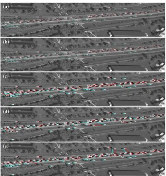
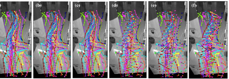
We test our object tracking method and multi-graph matching method on several datasets, such as the MOT16 challenge benchmark. For different datasets or dif-ferent applications, difdif-ferent affinities between objects are defined. For example, on the MOT16 challenge benchmark dataset, the affinities are defined using the features from
deep siamese neural networks. It is shown that our methods have excellent performance in comparison with the state of the art.
The remainder of the paper is organized as follows: Sect. 2 briefly introduces rank-1 tensor approximation. Section 3 describes the dual L1-normalized rank-1 tensor approximation. Sections 4 and 5 propose context and hyper-context aware tensor power iterations. Sections 6 and 7 pre-sent our multi-object tracking method and our multi-graph matching method respectively. Section 8 demonstrates the experimental results. Section 9 summarizes the paper.
2 Rank‑1 Tensor Approximation
A tensor is the high dimensional generalization of a matrix. Each element in a K-order tensor A∈ℝI1×⋯×Ik⋯IK is
repre-sented as ai
1⋯ik−1ikik+1⋯iK where 1≤ik≤Ik . Each order of a
tensor is associated with a mode. The k-mode product of a tensor A∈ℝI1×⋯×Ik−1×Ik×Ik+1⋯IK and a matrix 𝐖∈ℝIk×Jk is a
new tensor B∈ℝI1×⋯×Ik−1×Jk×Ik+1⋯IK whose entries are
This k-mode product is notated as B=A⊗k𝐖 . In
particu-lar, the k-mode product of A and a vector 𝐰∈ℝIk is a K −1
order tensor:
A rank-1 tensor Ĉ ∈ℝI1×⋯×Ik−1×Ik×Ik+1⋯IK is a specific
ten-sor which can be represented as the outer product ( ∗ ) of
K vectors { ̂𝐰k∈ℝIk}K
k=1 : Ĉ= ̂𝐰
1∗ ̂𝐰2
⋯𝐰̂k⋯∗ ̂𝐰K , i.e., an
element in Ĉ is represented as:
where ŵki
k is the ik th element in ̂
𝐰k . Let {𝐰k∈ℝIk}K k=1 be K L2 unit-normalized column vectors and let W be the matrix composed of {𝐰k∈ℝIk}K
k=1 . A rank-1 approximation to a
tensor A∈ℝI1×⋯×Ik−1×Ik×Ik+1⋯IK is obtained by finding the
vectors {𝐰k∈ℝIk}K
k=1 and a scalar 𝛾 for minimizing the
fol-lowing square of the Frobenius norm:
(1)
bi
1⋯ik−1jkii+1iK =
Ik
∑
ik=1
ai
1⋯ik−1ikik+1⋯iKwikjk.
(2)
(A⊗k𝐰)i1⋯ik−1ii+1iK =
Ik
∑
ik=1 ai
1⋯ik−1ikik+1⋯iKwik.
(3)
̂
ci
1…ik…iK= ( ̂𝐰
1∗ … ∗ ̂𝐰k… ∗ ̂𝐰K)
i1⋯ik⋯iK = ̂w
1 i1ŵ
2 i2⋯ŵ
k ik⋯ŵ
K iK,
(4)
min 𝛾,𝐖‖‖‖
A− 𝛾𝐰1∗ 𝐰k⋯∗ 𝐰K‖‖‖
2
F
=min
𝛾,𝐖
I1
∑
i1=1
I2
∑
i2=1
⋯ IK
∑
iK=1 (
ai
1i2⋯iK− 𝛾 w1
i1w
2
i2⋯w K iK
By solving (4), the tensor A is approximated by the rank-1
tensor 𝛾𝐰1∗ 𝐰k
⋯∗ 𝐰K . A function g is defined as:
With some derivations as shown in Regalia and Kofidis (2000), De Lathauwer et al. (2000), the optimization in (4) has the following equivalent form:
Tensor power iteration (Regalia and Kofidis 2000; De Lathauwer et al. 2000) has been proposed to optimize (6).
3 Dual
L
1‑Normalized Rank‑1 Tensor
Approximation
Many applications, such as multi-frame data association and multi-graph matching, can be formulated as multi-dimen-sional assignment problems (Collins 2012). We transform the multi-dimensional assignment problem to a rank-1 ten-sor approximation problem. Then, mathematical techniques for rank-1 tensor approximation are introduced to solve the multi-dimensional assignment problem.
3.1 Formulation
Suppose that there is a sequence of K + 1 sets of samples and each set has N samples.1 Let i
k be a sample index in the kth
set. A trajectory i0i1i2⋯iK is a sequence of K + 1 samples
from the K + 1 sets respectively (we index sample sets stat-ing from 0 for description convenience). Let ai
0i1i2⋯iK be the
affinity of trajectory i0i1⋯iK whose label xi0i1⋯iK is 1 if the
trajectory is actually existent, otherwise is 0. An actually existent trajectory has higher affinity between the samples in it. Multi-dimensional assignment is formulated as:
(5)
g(𝐰1 ,𝐰2
,…,𝐰K
) =||
|A⊗1𝐰 1⊗
2𝐰 2
⋯⊗K𝐰
K|| |
=
I1 ∑
i1=1 I2 ∑
i2=1 ⋯
IK ∑
iK=1
ai
1i2⋯iK
w1i
1
w2i
2⋯
wKi
K .
(6)
max
𝐖 g(𝐰
1
,𝐰2,…,𝐰K).
(7)
max
N ∑
i0=1
N ∑
i1=1
⋯ N ∑
iK=1
ai
0i1⋯iKxi0i1⋯iK,
(8)
s.t. ⎧ ⎪ ⎨ ⎪ ⎩
xi
0i1…iK∈ {0, 1}, 0≤k≤K;
∀ik∈ {1, 2,…,N}, N
∑
i0=1
N
∑
i1=1
⋯
N
∑
ik−1
N
∑
ik+1
⋯
N
∑
iK=1
xi
0i1⋯ik⋯iK=1.
Actually existent trajectories are found by solving this con-strained integer optimization.
We decompose a global association xi
0i1⋯iK into a
sequence of pairwise associations:
where xik
k−1,ik ∈ {0, 1} is the association between the ik−1 th
sample in the k-1th set and the ik th sample in the kth set.
Only if all the pairwise associations in the sequence are true (i.e., take value 1), is the global association also true. It is apparent that there are N2 associations between two
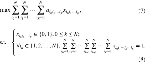
consecu-tive sample sets. In order to transform multi-dimensional assignment to a rank-1 tensor approximation problem, we flatten (unfold) the association matrix [xk
ik−1,ik ]
N×N between
the k-1th sample set and the kth sample set into a vector
[
wk𝝑
k ]N2
𝝑k=1 . To more clearly distinguish the association matrix
and the flattened association vector, we use bold italic font to indicate the elements in an association vector. The relation between the association matrix and the association vector is illustrated in Fig. 1. The equivalent relation between the association index 𝝑k in the vector and the indices ik−1 and ik
in the association matrix is:
(9)
xi0i1⋯iK =x
1 i0,i1x
2 i1,i2⋯x
K iK−1,iK,
(10)
𝝑k= (ik−1−1)N+ik.
Fig. 1 The relation between the association matrix and the
associa-tion vector: The sample associaassocia-tion (ik,ik+1) between two consecutive
sets k and k + 1 is represented by vector 𝜗k+1 ∈RN×N
. The upper part shows all the possible associations between three consecutive sets; the lower part shows the corresponding vector representation. The relation between the second sample in set 0 and the first sample in frame 1 (i0=2,i1=1) corresponds to the fourth element 𝜗1
4 in asso-ciation vector 𝜗1 ; The association (i
1=1,i2=3 )
corresponds to the third element 𝜗2
3 in association vector 𝜗
2
1 We assume that there is the same number of samples in each set.
[image:6.595.51.290.555.661.2]In this way, an association indexed by (ik−1,ik) in the
associa-tion matrix [xk ik−1,ik
]
N×N is also indexed by 𝝑k in the
associa-tion vector 𝐰k=(wk
𝝑k
)N2
𝝑k=1 :
xk ik−1,ik =
wk
𝝑k.
We rearrange the affinity ai
0i1i2⋯iK using the indices in
association vectors {𝐰k} . In the k-1th set the i
k−1 index of
the sample included in the association 𝝑k is ⌈𝝑k∕N⌉ , where
⌈ ⌉ is the up rounding operator; and in the kth set the index ik of the sample included in the 𝝑k th association is
𝝑k−
�
⌈𝝑k∕N⌉−1
�
N:
The consecutive associations 𝝑k and 𝝑k+1 have affinity
only if they share the same sample in the kth set. Then, we define the affinity s𝝑
1𝝑2⋯𝝑K of the global association
con-sisting of the consecutive pairwise associations {𝝑k}Kk=1 as
follows:
where 𝝑k−
�
⌈𝝑k∕N⌉−1
�
N= �𝝑k+1∕N �
means that asso-ciations 𝝑k and 𝝑k+1 share the same sample in the kth sample
set.
Using the pairwise association vectors {𝐰k}K k=1 and
the affinities defined on {𝐰k}K
k=1 , we can transform
multi-dimensional assignment to rank-1 tensor approximation. Let 𝐖∈ℝN2×K be the matrix composed of {𝐰k}K
k=1 . Using
(10) and (12), the objective of multi-dimensional assignment formulated in (7) is transformed to the objective of rank-1 tensor approximation:
The global constraint in (8) is decomposed into the following local pairwise constraints:
where xk
ik−1,ik is an element in the association matrix and it is
equal to wk𝝑
k . The dual L1 norm in (14) is that both the rows and
(11)
�
ik−1=⌈𝝑k∕N⌉,
ik=𝝑k− �
⌈𝝑k∕N⌉−1 �
N.
(12)
s
𝝑1𝝑2⋯𝝑K=
⎧ ⎪ ⎨ ⎪ ⎩ ai
0i1⋯iK
if 𝝑k−�⌈𝝑k∕N⌉−1�N=�𝝑k+1∕N
�
,
k=1, 2,…K−1
0 otherwise.
(13)
max 𝐖
g(𝐰1
𝝑1 ,𝐰2
𝝑2 ,…,𝐰K
𝝑K)
=max
𝐖 N2 ∑
𝝑1=1 N2 ∑
𝝑2=1 ⋯
N2 ∑
𝝑K=1
s𝝑
1𝝑2⋯𝝑K w1
𝝑1
w2 𝝑2⋯
wK 𝝑K . (14) ⎧ ⎪ ⎪ ⎨ ⎪ ⎪ ⎩ N ∑ ik−1=1
xk ik−1,ik =1
N ∑ ik=1
xk ik−1,ik =1
1≤k≤K,
columns in the association matrix [xk ik−1,ik
]
N×N are L1
-normal-ized. This ensures that one sample in the current set associates with only one sample in the subsequent set, and one sample in the subsequent set associates with only one sample in the cur-rent set. The optimization objective in (13) is the same as in (6). However, the original rank-1 tensor approximation in (6) is constrained by the L2 norm, while the optimization in (13) is constrained by the dual L1 norm. The methods for the origi-nal rank-1 tensor approximation are not suitable for solving the dual L1 normalized rank-1 tensor approximation.
3.2 Solution
We carry out the optimization in (13) by an iterative algo-rithm that finds the association variables {wk
𝝑k}
k=1,…,K
𝝑k=1,…,N2 . In
each iteration some association variables are updated while the remaining association variables are fixed. It is required that in each iteration the value of the objective function is increased.
A power iteration method is utilized to adapt the dual L1
unit norm constraint. The integer constraint on wk𝝑
k is relaxed
to a real value constraint: 0≤wk𝝑 k
≤1 . Then, wk𝝑
k represents
the probability of the association between the ik−1 th sample
in the k-1th set and the ik th sample in the kth set. A tensor
power is used to iteratively update 𝐰k= {wk
𝝑k}
N2
𝝑k=1 followed
by a dual L1 unit normalization. The iteration is based on the partial differential of g(𝐰1
,…,𝐰k
,𝐰k+1,…,𝐰K) for each
association vector element wk
𝝑k:
Let 𝐰k(𝜏) be the kth association vector at the 𝜏 th iteration. It
has elements {wk 𝝑k(𝜏)}
N2
𝝑k=1 . At the 𝜏 +1 th iteration, on
con-sidering the update of 𝐰k(𝜏) , with all other association
vec-tors {𝐰1(𝜏 +1),…,𝐰k−1(𝜏 +1),𝐰k+1(𝜏),…,𝐰K(𝜏)} fixed,
the following equations are used to update 𝐰k:
(15)
𝜕g(𝐰1,…,
𝐰k,𝐰k+1,…,
𝐰K)
𝜕wk
𝝑k
=
N2
∑
𝝑1=1
⋯
N2
∑
𝝑k−1=1 N2
∑
𝝑k+1=1
⋯
N2
∑
𝝑K=1
s𝝑
1⋯𝝑k⋯𝝑Kw
1 𝝑1⋯w
k−1 𝝑k−1w
k+1 𝝑k+1⋯
wK
𝝑K .
(16)
wk
𝝑k(𝜏 +1)
←wk𝝑k(𝜏)
N2
∑
𝝑1=1 ⋯
N2
∑
𝝑k−1=1 N2
∑
𝝑k+1=1
⋯
N2
∑
𝝑K=1
s𝝑 1𝝑2⋯𝝑K
w1
𝝑1(𝜏 +1)
⋯wk𝝑−k−11(𝜏 +1) wk+1
𝝑k+1(𝜏)⋯
wK
where (17) and (18) carry out the dual L1 normalization corresponding to the constraint in (14), ensuring the one to one mapping between samples in consecutive sets. We can prove that
The convergence shown in (19) ensures that (16), (17), and (18) form an effective iteration algorithm for solving the dual L1 normalized rank-1 tensor approximation problem. The original rank-1 tensor approximation in Sect. 2, con-strained by the L2 unit norm, has been proved to converge. In the following, we first prove that the iteration for the rank-1 tensor approximation constrained by the L1 unit norm is con-vergent, and then give the proof of convergence of the dual
L1 normalized rank-1 tensor approximation.
Proposition A For the L1normalized rank-1 tensor
approx-imation, each elementw1i
1in𝐰
1is updated by:
whereC1is the L
1normalization factor of𝐰1(𝜏 +1):
Then, we have
Namely, with the L1 normalized 𝐰1(𝜏 +1) , the iteration
using (20) converges.
Proof We define two temporary vectors 𝐆= (f1,f2,…,fI1)
and 𝐔= (u1,u2,…,uI1):
(17)
xki
k−1,ik(𝜏 +1)←
xk
ik−1,ik(𝜏 +1) ∑N
lk=1x k
ik−1,lk(𝜏 +1) ,
(18)
xki
k−1,ik(𝜏 +1)←
xk
ik−1,ik(𝜏 +1) ∑N
lk−1=1x
k
lk−1,ik(𝜏 +1)
,
(19)
g(𝐰1 𝝑1(
𝜏+1),…,𝐰k
𝝑k(𝜏+1),
𝐰k𝝑+1 k+1(𝜏) …
,𝐰K𝝑 K(𝜏))
≥g(𝐰1𝝑 1(𝜏+
1),…,
𝐰k 𝝑k(𝜏),𝐰
k+1
𝝑k+1(𝜏),…,𝐰 K 𝝑K(𝜏)).
(20)
w1i
1(𝜏 +1) = 1
C1w 1
i1(𝜏) I2
∑
i2=1
⋯
IK
∑
iK=1
ai
1i2⋯iKw
2
i2(𝜏)⋯w K iK(𝜏),
(21)
C1=
I1 ∑
i1=1
w1i
1(𝜏)
I2 ∑
i2=1 ⋯
IK
∑
iK=1
ai
1i2⋯iKw
2
i2(𝜏)⋯w
K iK(𝜏).
(22)
g(𝐰1(𝜏 +1),𝐰2(𝜏),…,𝐰K(𝜏))≥g(𝐰1(𝜏),𝐰2(𝜏),…,𝐰K(𝜏)).
Then, the following equation holds
where ‘ ⟨,⟩ ’ and ‘◦’ denote the inner product and the
Had-amard product (element-wise product) respectively. With the
L1 norm constraint ‖𝐔‖22=��𝐰1(𝜏)��
1=1 , the application of
the Cauchy–Schwarz inequality to (24) yields
After 𝐰1 is iterated using (20), the objective function is
rep-resented as:
It is apparent that
By combining formulae (25), (26), and (27), we prove the inequality (22). The convergence for the iterations of 𝐰2 , …,
and 𝐰K can be proved in the same way as for 𝐰1.
(23) ⎧ ⎪ ⎨ ⎪ ⎩ fi 1 = I2 ∑
i2=1 ⋯
IK
∑
iK=1 ai
1i2⋯iKw
2
i2(𝜏)⋯w
K iK(𝜏),
ui
1×ui1=w 1
i1(𝜏).
(24)
g(𝐰1(𝜏),𝐰2(𝜏),…,𝐰K(𝜏))
= I1
�
i1=1
I2
�
i2=1
⋯ IK �
iK=1 ai
1i2⋯iKw 1
i1(𝜏)w
2
i2(𝜏)⋯w K iK(𝜏)
= I1
�
i1=1
I2
�
i2=1
⋯ IK
�
iK=1 ai
1i2⋯iKui1ui1w
2
i2(𝜏)⋯w K iK(𝜏)
= I1
�
i1=1 ui1ui1
I2
�
i2=1
⋯ IK
�
iK=1
ai1i2⋯iKw 2
i2(𝜏)⋯w K iK(𝜏)
=⟨𝐔,𝐔◦𝐆⟩
(25)
g(𝐰1(𝜏),𝐰2(𝜏),…,𝐰K(𝜏)) =⟨𝐔,𝐔◦𝐆⟩≤‖𝐔‖
2‖𝐔◦𝐆‖2=‖𝐔◦𝐆‖2.
(26)
g(𝐰1(𝜏 +1),𝐰2(𝜏),…,𝐰N(𝜏))
=� i1 � i2 ⋯ � iK
ai1i2⋯iKw 1
i1(𝜏 +1)w
2
i2(𝜏)⋯w K iK(𝜏)
=�𝐰1(𝜏 +1),𝐆�= 1
C1
�
𝐰1(𝜏),𝐆�
= 1
C1
�
𝐰1(𝜏)◦𝐆,𝐆�
= 1
C1⟨𝐔◦𝐆,𝐔◦𝐆⟩=
1
C1‖𝐔◦𝐆‖ 2 2.
(27)
C1=
I
1
∑
i
1=1
w1i
1 (𝜏) I 2 ∑ i
2=1
⋯ IK ∑
iK=1
ai
1i2⋯iKw
2 i
2
(𝜏)⋯wKi K
(𝜏)
Proposition B For the dualL1-normalized rank-1 tensor approximation, the following equations are used to update 𝐰1.
where (29) and (30) carry out the dual L1normalization.
Then, we have
Proof Similar to the definition of G using (23), we define a vector 𝐆= (f1,f2,…,fN2) as follows:
Let 𝐆i0∈ℝ1×N= (fi0,1,fi0,2,…,fi0,N)(1≤i0≤N ), where
{i0,j}Nj=1 are defined using (11). Set 𝐆= {𝐆i0}
N i0=1 . The
objective function is represented as:
The objective function is the sum of N components
⟨
𝐰i0,𝐆i0 ⟩
. Each component ⟨𝐰i0,𝐆i0
⟩
corresponds to a L1
normalized rank-1 tensor approximation whose iteration convergence is proved in Proposition A. Therefore, the itera-tions in (28), (29) and (30) for the dual L1-normalized rank-1 tensor approximation also converge. The convergence for the iterations of 𝐰2 , …, and 𝐰K can be proved in the same
way as for 𝐰1.
3.3 Discussion
In the solution, it is assumed that the sample sets have the same number of samples. When different numbers of sam-ples exist in different sample sets, virtual samsam-ples are added to sample sets to make the number of samples in each set the same. The affinities to virtual samples are set to a fixed small (28)
w1
𝝑1(𝜏 +1)←w
1
𝝑1(𝜏)
N2
∑
𝝑1=1
N2
∑
𝝑2=1
⋯
N2
∑
𝝑K=1
s𝝑1𝝑2⋯𝝑
Kw 2
𝝑2(𝜏)⋯w
K
𝝑K(𝜏)
(29)
x1i
0,i1(𝜏 +1)← x1
i0,i1(𝜏 +1)
∑N
l1=1x 1
l0,l1(𝜏 +1)
,
(30)
x1i
0,i1(𝜏 +1)←
x1
i0,i1(𝜏 +1) ∑N
l0=1x 1
l0,l1(𝜏 +1)
,
(31)
g(𝐰1
𝝑1(𝜏 +1),𝐰 2
𝝑2(𝜏),…,𝐰
K
𝝑K(𝜏))≥g(𝐰 1 𝝑1(𝜏),𝐰
2
𝝑2(𝜏),…,𝐰
K
𝝑K(𝜏)).
(32)
f𝝑 1=
N2
∑
𝝑2=1 ⋯
N2
∑
𝝑K=1 s𝝑
1𝝑2⋯𝝑Kw
2
𝝑2(𝜏)⋯w
K
𝝑K(𝜏) (1≤𝝑1≤N 2
).
(33)
g(𝐰1(𝜏 +1),𝐰2(𝜏),…,𝐰K(𝜏)) =⟨𝐰1((𝜏 +1),𝐆⟩=
N
∑
i0=1
⟨ 𝐰i0,𝐆i0
⟩ .
value. This fixed small value corresponds to the probability that samples appear or disappear. The same small affinity of the virtual samples in a set to the samples in other sets ensures that the virtual samples do not influence the match-ing of the non-virtual samples in the sets. After finalization of association, the isolated samples in one set are associated with the virtual samples in other sets.
The above tensor formulation has various applications, depending on the form of the elements s𝝑
1⋯𝝑k⋯𝝑K in the tensor.
In particular, two applications are 2D assignment and network flow. If s𝝑1⋯𝝑k⋯𝝑K is decomposed as the sum of pairwise
affini-ties: s𝝑1⋯𝝑k⋯𝝑K =
∑K k=1s
k
𝝑k , where s
k
𝝑k denotes the affinity of
the 𝝑k th association between the k-1th sample set and the kth
sample set, then the objective in (13) is reformulated as:
NK−1∑K
k=1 ∑N2
𝝑k=1s
k
𝝑kw
k
𝝑k . This optimization corresponds to
the 2D assignment problem. When the affinity is computed as the product of pairwise affinities: s𝝑1⋯𝝑k⋯𝝑K =
∏K k=1s
k
𝝑k , the
objective in (13) is rewritten as ∏Kk=1
∑N2 𝝑k=1s
k
𝝑kw
k
𝝑k . This
objective is appropriate for network flow (Berclaz et al. 2011). As a result, tensor approximation provides a flexible frame-work to take advantage of global and local association affini-ties. However, the above tensor approximation does not encode context information between trajectories.
4 Context‑Aware Tensor Power Iteration
Contexts between samples can be used to reduce the unre-liability of sample associations. For example, the moving vehicles in a local spatiotemporal space usually have simi-lar motion patterns. The determination of the association for a vehicle can be improved using the motion information about other vehicles. We combine the pairwise contextual relations between associations into the optimization objec-tive and propose a dual L1-normalized context-aware tensor power iteration algorithm to determine the relations between samples.
Let ck𝝑
k𝝇k be the contextual affinity between two
associa-tions indicated by wk
𝝑k and w
k
𝝇k respectively. Embedding the
contextual affinity into the temporal affinity in (13) yields a joint optimization which is a linear combination of the tem-poral affinity and the contextual affinity:
(34) max 𝐖 ⎛ ⎜ ⎜ ⎝ N2 �
𝝑1=1 ⋯
N2
�
𝝑k=1 ⋯
N2
�
𝝑K=1 s𝝑
1⋯𝝑k⋯𝝑Kw
1 𝝑1⋯
wk
𝝑k⋯ wK
𝝑K
+𝛼
K �
k=1 N2
�
𝝑k=1
N2
�
𝝇k=1 ck
where α is a weighting parameter which is used to balance the effects of the two affinities, and the second term models the contexts between associations. The optimization is also constrained by (14) as well as 0≤wk𝝑
k ≤1.
The new optimization in (34) is more difficult than the basic one in (13) due to the quadratic contextual term. We make some reformulations to (34) to make it solvable by iterations. From (14), it is apparent that
By using (35), the first term in (34) is rewritten as follows:
By using (35), the second term in (34) is rewritten as follows:
where wk
𝝑k is not included in the continued multiplication
∏
f≠k
because it already exists in the preceding term. Merging (36) and (37), the optimization (34) is rewritten as:
We apply the block update strategy (Collins 2012) to opti-mize (38) iteratively. Namely, when the block variables in
𝐰k are updated to yield a local optimization, other block
(35)
1
N
N2 ∑
𝝇k=1
wk𝝇
k =1, k=1, 2,…,K.
(36) N2 � 𝝑1=1 ⋯ N2 � 𝝑k ⋯ N2 �
𝝑K=1
s𝝑1⋯𝝑 k⋯𝝑Kw
1
𝝑1⋯w k 𝝑k⋯w
K 𝝑K = ⎛ ⎜ ⎜ ⎝ 1 N N2 �
𝝇k=1 wk𝝇
k ⎞ ⎟ ⎟ ⎠ N2 �
𝝑1=1
⋯
N2
�
𝝑k=1
⋯
N2
�
𝝑K=1 s𝝑
1⋯𝝑k⋯𝝑Kw 1
𝝑1⋯w k 𝝑k⋯w
K 𝝑K = 1 N N2 � 𝝑1=1 ⋯ N2 � 𝝑k=1 N2 �
𝝇k=1
⋯
N2
�
𝝑K=1
s𝝑1
⋯𝝑k⋯𝝑Kw 1
𝝑1⋯
wk 𝝑k
wk 𝝇k⋯
wK 𝝑K.
(37)
N2 �
𝝑k=1
N2 �
𝝇k=1
ck𝝑
k𝝃kw
k
𝝑kw
k
𝝇k =
⎛ ⎜ ⎜ ⎝ N2 �
𝝑k=1
N2 �
𝝇k=1
ck𝝑
k𝝇kw
k
𝝑kw
k 𝝇k ⎞ ⎟ ⎟ ⎠ � f≠k ⎛ ⎜ ⎜ ⎝ 1 N N2 �
𝝑f=1
wf𝝑f
⎞ ⎟ ⎟ ⎠
= 1
NK−1 N2 �
𝝑1=1
⋯
N2 �
𝝑k=1 N2 �
𝝇k=1
⋯
N2 �
𝝑K=1
ck𝝑
k𝝇kw
1
𝝑1⋯w k
𝝑kw
k
𝝇k⋯w
K
𝝑K,
(38)
max N2 �
𝝑1=1
⋯ N2 �
𝝑k=1
⋯ N2 �
𝝑K=1
s 𝝑1⋯𝝑k⋯𝝑Kw
1
𝝑1⋯
w2
𝝑k⋯w K 𝝑K
+ 𝛼
N2 �
𝝑k=1
N2 �
𝝇k=1
ck 𝝑k𝝇kw
k 𝝑kw
k 𝝇k+ 𝛼
�
f≠k N2 �
𝝑f=1
N2 �
𝝇f=1
cf 𝝑f𝝇fw
f 𝝑fw
f 𝝇f
=max1 N
N2 �
𝝑1=1
⋯ N2 �
𝝑k=1
N2 �
𝝇k=1
⋯ N2 �
𝝑K=1
⎛ ⎜ ⎜ ⎝ s𝝑
1⋯𝝑k⋯𝝑K+
𝛼ck 𝝑k𝝇k NK−2
⎞ ⎟ ⎟ ⎠ w1
𝝑1⋯
wk 𝝑kw
k 𝝇k⋯w
K 𝝑K
+ 𝛼�
f≠k N2 �
𝝑f=1
N2 �
𝝇f=1
cf 𝝑f𝝇fw
f 𝝑fw
f 𝝇f.
variables {𝐰f|f ≠k} are fixed. In this way, the complicated
optimization in the global space reduces to a simplified solu-tion in a local space. The second term in the right hand of the equality sign in (38) can be omitted. Thus, the optimization (38) reduces to:
The problem in solving (39) is that wk𝝑
k and w
k
𝝇k lie in the
same block vector 𝐰k and couple with each other. Namely,
when wk𝝑
k is updated, w
k
𝝇k cannot be fixed. To solve this
prob-lem, we decouple the interdependency between wk𝝑
k and w
k
𝝇k
to simplify the optimization. If two association hypotheses indicated by wk𝝑
k and w
k
𝝇k share the same object in the k-1th
sample set or in the kth sample set [i.e., ik−1=jk−1 or ik=jk ,
where the relation between jk−1 and 𝜁k is defined as in (11)],
then we set their contextual affinity ck𝝑
k𝝇k to 0. This is because
one sample does not exist in two real associations between two sample sets. Then, we reformulate (39) as follows:
Let el
1…lkjk…lK be the element of a (K + 1)-order augmented
tensor, which is defined as:
Then, (40) is transformed to:
In (42), (40) is decomposed into a series of the following optimizations:
In (43), the interdependency between wk 𝜗k and w
k
𝝇k is
decou-pled. The optimization in (43) has the same form with (13). Then, we can use the dual L1 normalized tensor power itera-tion method in Sect. 3 to solve (43).
In actual calculation, it is not necessary to construct the (K + 1)-order augmented tensor using (41). Instead we carry out the following iteration:
(39) max 𝐰k N2 ∑ 𝝑1=1 ⋯ N2 ∑
𝝑k=1
N2 ∑
𝝇k=1
⋯ N2 ∑
𝝑K=1
( s𝝑1⋯𝝑
k⋯𝝑K+
𝛼ck 𝝑k𝝇k
NK−2
) w1
𝝑1⋯ wk
𝝑k
wk 𝝇k⋯
wK 𝝑K . (40) max 𝐰k N2 ∑
𝝑1=1
⋯ N2
∑
𝝑k=1
∑
{𝝇k∶jk−1≠ik−1}
⋯ N2
∑
𝝑K=1
( N
N−1s𝝑1⋯𝝑k⋯𝝑K+ 𝛼ck
𝝑k𝝇k
NK−2
)
×w1𝝑
1⋯w
k 𝝑kw
k 𝝇k⋯w
K 𝝑K
.
(41)
e𝝑
1⋯𝝑k𝝇k⋯𝝑K =
N
N−1s𝝑1⋯𝝑k⋯𝝑K+ 𝛼ck
𝝑k𝝇k
NK−2.
max
𝐰k
N2
∑
𝝑1=1
⋯
N2
∑
𝝑k=1 ∑
𝝇k≠𝝑k ⋯
N2
∑
𝝑K=1
e𝝑1⋯𝝑k𝝇k⋯𝝑Kw 1
𝝑1⋯w
k 𝝑kw
k 𝝇k⋯w
K 𝝑K
=
N
∑
ik=1 max
𝐰k
N2
∑
𝝑1=1 ⋯
N2
∑
𝝑k=1 ∑
{𝝇k∶jk−1≠ik−1} ⋯
N2
∑
𝝑K=1
e𝝑1⋯𝝑k𝝇k⋯𝝑Kw 1
𝝑1⋯w
k 𝝑kw
k 𝝇k⋯w
K 𝝑K . (43) max 𝐰k N2 ∑
𝝑1=1 ⋯
N2
∑
𝝑k=1 ∑
{𝝇k∶jk−1≠ik−1} ⋯
N2
∑
𝝑K=1
e𝝑1⋯𝝑k𝛓k⋯𝝑Kw
1
𝝑1⋯w
k 𝝑kw
k
𝝇k⋯w
K 𝝑K.
It is seen that in the iteration the computation only involves the pairwise associations including the current (44)
wk 𝝑k(𝜏 +
1)
∝wk 𝝑k(𝜏)
N2 ∑
𝝑1=1 ⋯
∑
{𝝑f|f≠k}
⋯
N2 ∑
𝝑K=1 ∑
{𝝇k|jk≠ik}
e𝝑1⋯𝝑k𝝇k⋯𝝑Kwk𝝇kw 1 𝝑1⋯w
k 𝝑f⋯w
K 𝝑K
∝wk𝝑k(𝜏) N2 ∑
𝝑1=1 ⋯
∑
{𝝑f|f≠k}
⋯
N2 ∑
𝝑K=1
s𝝑1⋯𝝑k⋯𝝑Kw 1 𝝑1⋯w
k 𝝑f⋯w
K 𝝑K
+ ∑
{𝝇k|jk−1≠ik−1} ck
𝝑k𝝇kw k 𝝇k.
set k. While the computational complexity of the itera-tion in the dual L1 normalized tensor power iteration is O(N2K) , the computational complexity in (44) is O(N2K+N2) =O(N2K) as O(N2K) ≫O(N2) . Considering
the contexts only slightly increases the runtime. The dual
two objects from two consecutive frames respectively is generated only when they are spatially close to each other. Removing unnecessary association hypotheses in this way greatly reduces the computational complexity and storage space. In a scene, moving objects may enter, exit, reappear, be occluded, or be missed, etc. There may be detections that have no associated detection in consecutive frames. To han-dle this issue, virtual detections are introduced in each frame to drop out the isolated detections and thus avoid disturb-ing the real detection associations. Appearance models and motion models are used to construct the temporal affinity. The contextual affinity is defined using motion contexts. The context-aware tensor power iteration is applied to obtain the real valued associations between detections. The real valued solutions must be discretized to meet the integer and one-to-one mapping constraints in the assignment. We regard the real valued solutions as the costs for the corresponding associations, and apply the Hungarian algorithm to obtain the binary association outputs. In the following, we detail tensor construction, definition of the contextual affinity, and the computational complexity analysis.
6.1 Tensor Construction
The form of the elements s𝝑
1⋯𝝑k⋯𝝑K in (34) depends on the
application and the particular temporal affinities. In some applications the temporal affinities are based on motion models while in other applications it is necessary to com-bine appearance models and motion models to define the temporal affinity. Two methods for defining temporal affini-ties are described.
The first method defines the temporal affinity of a trajec-tory based on a global motion affinity m𝝑
1𝝑2⋯𝝑K and
appear-ance affinities given by associations between consecutive frames. Let 𝐳k
𝝑k = �������������⃗𝕆
k−1
ik−1
𝕆k
ik be the spatial displacement of the
association between objects 𝕆k−1
ik−1 at frame k −1 and 𝕆
k ik at
frame k. If objects 𝕆k−1
ik−1 and
𝕆k
ik are the same object, 𝐳
k
𝝑k is the
velocity vector of the object. The global motion affinity is defined as:
where the first part in the exponential term is the cosine of two velocity vectors measuring their direction consistency and the second part measures their amplitude consistency. This motion affinity describes object motion inertia: an object has similar velocities in consecutive frames. For an object 𝕆k
ik , we use a gray scale histogram {h
1 ik,h
2
ik,…} and the
area bk
ik of the box bounding the object to represent its
(51)
m𝝑
1𝝑2⋯𝝑K =
K−1 �
k=1
exp ⎛ ⎜ ⎜ ⎜ ⎝ (𝐳k
𝝑k)
T𝐳k+1
𝝑k+1 ��
�𝐳k𝝑k���2���𝐳 k+1
𝝑k+1���2
+ 2��
�𝐳k𝝑k���2���𝐳
k+1
𝝑k+1���2
�� �𝐳k𝝑k���
2
2+���𝐳 k+1
𝝑k+1��� 2 2 ⎞ ⎟ ⎟ ⎟ ⎠ ,
5 Hyper Context‑Aware Power Iteration
We replace the pairwise contexts formulated in Sect. 4 with hyper-contexts among triples of associations. Suppose that
wk𝝑 k ,
wk 𝝇k , w
k
𝝊k represent, respectively, the associations on
sam-ples pairs 𝕆k−1
ik−1 ↔
𝕆k ik ,
𝕆k−1
jk−1 ↔
𝕆k jk , and
𝕆k−1 lk−1 ↔
𝕆k
lk between
the k-1th sample set and the kth sample set. The affinity of the hyper-context among wk𝝑
k , w
k
𝝇k , and w
k
𝝊k is represented as
ck𝝑
k𝝇k𝝊k . By replacing the context affinity with the
hyper-con-text affinity, the objective of hyper-conhyper-con-text aware tensor approximation is extended as:
Using tensor power iteration to solve the above optimiza-tion, we only need to replace (46) with
6 Multi‑object Tracking
Multi-object tracking can be carried out in a batch or online mode:
• Batch mode For a batch of K + 1 successive frames,
N objects in each frame are detected, and N2
associa-tion hypotheses are generated between two consecutive frames. Then, a K order tensor is constructed by com-puting the temporal affinity. The context affinities are computed. Based on these affinities, the dual L1 norm context-aware tensor power iteration is applied to find the real associations between the detected objects. After that, the next batch of K + 1 successive frames is processed in the same way as for the preceding batch, where the two batches share a common boundary frame. Serial expan-sion of the associations in all the batches in a video yields the global trajectories of the detected objects.
• Online mode Given a new frame, it is combined with the
preceding K frames. The dual L1 normalized context-aware tensor power iteration is applied to find the object associations between these K + 1 frames.
The main components of the multi-object tracking algo-rithm include association hypothesis generation, tensor con-struction, definition of the contextual affinity, and initiali-zation and termination. An association hypothesis between
(49)
max
𝐖
N2 ∑
𝝑1=1 ⋯
N2 ∑
𝝑k=1 ⋯
N2 ∑
𝝑K=1 s𝝑
1⋯𝝑k⋯𝝑K w1
𝝑1⋯ wk
𝝑k⋯ wK
𝝑K
+𝛼
K
∑
k=1
N2 ∑
𝝑k=1
N2 ∑
𝝇k=1
N2 ∑
𝝊k=1 ck
𝝑k𝝇k𝝊k wk 𝝑k wk 𝝇k wk 𝝊k . (50) 𝜓i
k−1,ik = ∑
{𝝇k|jk−1≠ik−1} ∑
{𝝊k|lk−1≠ik−1}
ck𝝑
k𝝇k𝝊kw
k
𝝇kw
k