On Optimization of Manufacturing of Bipolar
Heterotransistors Framework Circuit of a High-voltage
Element or to Increase Their Integration Rate: On
Influence Mismatch-induced Stress
E. L. Pankratov1,2
1
Nizhny Novgorod State University, Russia 2
Nizhny Novgorod State Technical University, Russia
Copyright©2019 by authors, all rights reserved. Authors agree that this article remains permanently open access under the terms of the Creative Commons Attribution License 4.0 International License
Abstract
In this paper, we introduce an approach to decrease dimensions of bipolar heterotransistors framework a circuit of a voltage divider biasing common emitter amplifier. Framework of the approach, we consider manufacturing of the divider in heterostructure with specific configuration. Several specific areas of the heterostructure should be doped by diffusion or by ion implantation. After this doping, dopant and/or radiation defects should be annealed by using optimized scheme. We also consider an approach to decrease value of mismatch-induced stress in the considered heterostructure. To make prognosis of technological process and obtain recommendations to optimize the process, we introduce an analytical approach to analyze mass and heat transport in heterostructures with account mismatch-induced stress.Keywords
Voltage Divider Biasing Common Emitter Amplifier, Increasing Integration Rate of Bipolar Transistors, Optimization of Manufacturing1. Introduction
In the present time, several actual problems of solid state electronics (such as increasing of performance, reliability and density of elements of integrated circuits: diodes, field-effect and bipolar transistors) are intensively solving [1-6]. To increase the performance of these devices, it is attracted an interest determination of materials with higher values of charge carriers mobility [7-10]. One way to decrease dimensions of elements of integrated circuits is
manufacturing them in thin film heterostructures [3-5, 11]. In this case, it is possible to use inhomogeneity of heterostructure to improve properties of considered devices. However, it is necessary to optimize doping of electronic materials [12, 13] and development of epitaxial technology to improve considered materials (including analysis of mismatch induced stress) [14-16]. An alternative approach to using heterostructures is using laser or microwave types of annealing [17-19].
Figure 1a. Structure of the considered voltage divider [13]
Figure 1b. Heterostructure with a substrate, epitaxial layers and buffer layer (view from side)
2. Method of Solution
To solve our aim, we determine and analyze spatio-temporal distribution of concentration of dopant in the considered heterostructure. We determine the distribution by solving of the second Fick's law in the following form [1, 20-24]
(
)
(
)
(
)
(
)
+
∂
∂
∂
∂
+
∂
∂
∂
∂
+
∂
∂
∂
∂
=
∂
∂
z
t
z
y
x
C
D
z
y
t
z
y
x
C
D
y
x
t
z
y
x
C
D
x
t
t
z
y
x
C
,
,
,
,
,
,
,
,
,
,
,
,
(
) (
)
+
∫
∇
∂
∂
Ω
+
S Sx
y
z
t
LzC
x
y
W
t
d
W
T
k
D
x
01
,
,
,
,
,
,
(1)
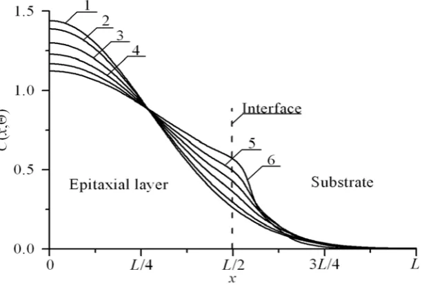
Here the first, the second and the third terms in right side of Eq. (1) describe thermal diffusion of dopant. The forth and the fifth terms of this equation describe transport of dopant under influence of mismatch-induced stress. Boundary (correspond to absents of dopant flow through external boundary of considered heterostructure) and initial conditions for Eq.(1) are
, , , C(x,y,z,0)=fC(x,y,z),
, , .
Function C(x,y,z,t) describes the spatio-temporal distribution of concentration of dopant; Ω is the atomic volume of dopant; ∇s is the symbol of surficial gradient; is the surficial concentration of dopant on interface
between layers of heterostructure (in this situation we assume, that Z-axis is perpendicular to interface between layers of heterostructure); µ1(x,y,z,t) is the chemical potential due to the presence of mismatch-induced stress; D and DS are the
coefficients of volumetric and surficial diffusions. Values of dopant diffusions coefficients depends on properties of materials of heterostructure, speed of heating and cooling of materials during annealing and spatio-temporal distribution of concentration of dopant. Dependences of dopant diffusions coefficients on parameters could be approximated by the following relations [22-24]
,
. (2)
Here the first multipliers in the right side of Eqs. (2) describe coefficient of linear diffusion. Nonlinearity of diffusion (in the high doped case [22]) was taken into account by the second multipliers in the Eqs. (2). The third multipliers of Eqs. (2) give a possibility radiation damage of materials of heterostructure [23,24]. Functions DL(x,y,z,T) and DLS(x,y,z,T) in
Eqs. (2) describe the spatial (due to accounting layers of heterostruicture) and temperature (due to Arrhenius law) dependences of dopant diffusion coefficients; T is the temperature of annealing; P(x,y,z,T) is the limit of solubility of dopant; parameter γ depends on properties of materials and could be integer in the following interval γ∈[1,3] [22]; V
(x,y,z,t) is the spatio-temporal distribution of concentration of radiation vacancies; V* is the equilibrium distribution of vacancies. Concentrational dependence of dopant diffusion coefficient has been described in details in [22]. Spatio-temporal distributions of concentration of point radiation defects have been determined by solving the following system of equations [20, 23, 24]
(
) (
)
∫
∇
∂
∂
Ω
+
LzS S
W
d
t
W
y
x
C
t
z
y
x
T
k
D
y
01
,
,
,
,
,
,
µ
(
)
0
,
,
,
0
=
∂
∂
= x
x
t
z
y
x
C
(
)
0
,
,
,
=
∂
∂
=Lx
x
x
t
z
y
x
C
(
)
0
,
,
,
0
=
∂
∂
= y
y
t
z
y
x
C
(
)
0
,
,
,
=
∂
∂
=Ly x
y
t
z
y
x
C
(
)
0
,
,
,
0
=
∂
∂
= z
z
t
z
y
x
C
(
)
0
,
,
,
=
∂
∂
=Lz
x
z
t
z
y
x
C
(
)
∫
zL
z
d
t
z
y
x
C
0
,
,
,
(
)
(
(
)
)
(
)
(
( )
)
+
+
+
=
2* 2 2 *
1
,
,
,
,
,
,
1
,
,
,
,
,
,
1
,
,
,
V
t
z
y
x
V
V
t
z
y
x
V
T
z
y
x
P
t
z
y
x
C
T
z
y
x
D
D
C Lξ
γς
ς
γ
(
)
(
(
)
)
(
)
(
( )
)
+
+
+
=
2* 2 2 *
1
,
,
,
,
,
,
1
,
,
,
,
,
,
1
,
,
,
V
t
z
y
x
V
V
t
z
y
x
V
T
z
y
x
P
t
z
y
x
C
T
z
y
x
D
D
S SLξ
S γς
ς
γ
(
)
(
) (
)
(
) (
)
+
+
=
y
t
z
y
x
I
T
z
y
x
D
y
x
t
z
y
x
I
T
z
y
x
D
x
t
t
z
y
x
I
I
I
∂
∂
∂
∂
∂
∂
∂
∂
∂
∂
,
,
,
,
,
,
,
,
,
,
,
,
,
,
,
(
) (
)
−
(
) (
)
−
(
)
×
+
k
x
y
z
T
I
x
y
z
t
k
x
y
z
T
z
t
z
y
x
I
T
z
y
x
D
z
I II,
,
,
,
,
,
IV,
,
,
,
,
,
,
,
,
, 2 ,∂
∂
∂
(3)
with boundary and initial conditions
, , , ,
, , , ,
, , , ,
I(x,y,z,0)=fI (x, y, z), V(x,y,z,0)=fV (x, y, z). (4)
Here I(x, y, z, t) is the spatio-temporal distribution of concentration of radiation interstitials; I* is the equilibrium distribution of interstitials; DI(x, y, z, T), DV(x, y, z, T), DIS(x, y, z, T), DVS(x, y, z, T) are the coefficients of volumetric and
surficial diffusions of interstitials and vacancies, respectively; kI, V (x, y, z, T), kI, I (x, y, z, T) and kV,V (x, y, z, T) are the
parameters of recombination of point radiation defects and generation of their complexes. The first, the second and the third terms in right side of Eqs.(3) describe thermal diffusion of point defects. The forth terms of Eqs.(3) describe generation of simple complexes of point defects (divacancies and diinterstitials; see, for example, [24] and appropriate references in this book). The fives terms of Eqs.(3) describe recombination of point defects. The sixth and the seventh terms of Eqs.(3) describe transport of point defects under influence of mismatch-induced stress. All boundary conditions correspond to absent of flow of defects through external boundary of the considered heterostructure.
Spatio-temporal distributions of divacancies ΦV(x, y, z, t) and diinterstitials ΦI(x, y, z, t) could be determined by
solving the following system of equations [20, 23, 24]
(
) (
)
(
) (
)
+
∫
∇
∂
∂
Ω
+
×
LzS
IS
x
y
z
t
I
x
y
W
t
d
W
T
k
D
x
t
z
y
x
V
t
z
y
x
I
0
,
,
,
,
,
,
,
,
,
,
,
,
µ
(
) (
)
∫
∇
∂
∂
Ω
+
LzS IS
W
d
t
W
y
x
I
t
z
y
x
T
k
D
y
0,
,
,
,
,
,
µ
(
)
(
)
(
)
(
)
(
)
+
+
=
y
t
z
y
x
V
T
z
y
x
D
y
x
t
z
y
x
V
T
z
y
x
D
x
t
t
z
y
x
V
V
V
∂
∂
∂
∂
∂
∂
∂
∂
∂
∂
,
,
,
,
,
,
,
,
,
,
,
,
,
,
,
(
)
(
)
−
(
) (
)
−
(
)
×
+
k
x
y
z
T
V
x
y
z
t
k
x
y
z
T
z
t
z
y
x
V
T
z
y
x
D
z
V VV,
,
,
,
,
,
IV,
,
,
,
,
,
,
,
,
, 2 ,∂
∂
∂
∂
(
) (
)
(
) (
)
+
∫
∇
∂
∂
Ω
+
×
LzS
VS
x
y
z
t
V
x
y
W
t
d
W
T
k
D
x
t
z
y
x
V
t
z
y
x
I
0
,
,
,
,
,
,
,
,
,
,
,
,
µ
(
) (
)
∫
∇
∂
∂
Ω
+
LzS
VS
x
y
z
t
V
x
y
W
t
d
W
T
k
D
y
0,
,
,
,
,
,
µ
(
)
0
,
,
,
0
=
= x
x
t
z
y
x
I
∂
∂
(
)
0
,
,
,
=
=Lx x
x
t
z
y
x
I
∂
∂
(
)
0
,
,
,
0
=
= y
y
t
z
y
x
I
∂
∂
(
)
0
,
,
,
=
=Ly
y
y
t
z
y
x
I
∂
∂
(
)
0
,
,
,
0
=
= z
z
t
z
y
x
I
∂
∂
(
,
,
,
)
0
=
=Lz
z
z
t
z
y
x
I
∂
∂
(
)
0
,
,
,
0
=
= x
x
t
z
y
x
V
∂
∂
(
)
0
,
,
,
=
=Lx x
x
t
z
y
x
V
∂
∂
(
)
0
,
,
,
0
=
= y
y
t
z
y
x
V
∂
∂
(
,
,
,
)
=
0
=Ly
y
y
t
z
y
x
V
∂
∂
(
)
0
,
,
,
0
=
= z
z
t
z
y
x
V
∂
∂
(
)
0
,
,
,
=
=Lz
z
z
t
z
y
x
V
∂
∂
(
)
(
)
(
)
(
)
(
)
+
Φ
+
Φ
=
Φ
Φ Φ
y
t
z
y
x
T
z
y
x
D
y
x
t
z
y
x
T
z
y
x
D
x
t
t
z
y
x
I II
I
I
∂
∂
∂
∂
∂
∂
∂
∂
∂
∂
,
,
,
,
,
,
,
,
,
,
,
,
,
(5)
with boundary and initial conditions
, , ,
, , ,
, , , (6)
, , ,
ΦI(x,y,z,0)=fΦI (x,y,z), ΦV(x,y,z,0)=fΦV (x,y,z).
Here DΦI(x,y,z,T), DΦV(x,y,z,T), DΦIS(x,y,z,T) and DΦVS(x,y,z,T) are the coefficients of volumetric and surficial
diffusions of simplest complexes of radiation defects; kI(x,y,z,T) and kV(x,y,z,T) are the parameters of decay of complexes
of radiation defects. The first, the second and the third terms in right side of Eqs.(5) describe thermal diffusion of simplest complexes of point defects. The forth and the fives terms of Eqs.(5) describe transport of divacancies and diinterstitials under influence of mismatch-induced stress. The sixth terms of Eqs.(5) describe generation of divacancies and diinterstitials. The seventh terms of Eqs.(5) describe decay of complexes of point radiation defects. All boundary conditions correspond to absent of flow of defects through external boundary of the considered heterostructure.
Chemical potential µ1 in Eq.(1) could be determine by the following relation [20]
µ1=E(z)Ωσij [uij(x,y,z,t)+uji(x,y,z,t)]/2, (7)
(
)
(
)
(
)
(
)
+
∫ Φ
∇
∂
∂
Ω
+
Φ
+
ΦΦ
z I
I
L I S
S I
W
d
t
W
y
x
t
z
y
x
T
k
D
x
z
t
z
y
x
T
z
y
x
D
z
01
,
,
,
,
,
,
,
,
,
,
,
,
µ
∂
∂
∂
∂
(
)
(
)
+
(
) (
)
+
∫ Φ
∇
∂
∂
Ω
+
Φt
z
y
x
I
T
z
y
x
k
W
d
t
W
y
x
t
z
y
x
T
k
D
y
IIL I S
S z
I
,
,
,
,
,
,
,
,
,
2,
,
,
, 0
1
µ
(
x
y
z
T
) (
I
x
y
z
t
)
k
I,
,
,
,
,
,
+
(
)
(
)
(
)
(
)
(
)
+
Φ
+
Φ
=
Φ
Φ Φ
y
t
z
y
x
T
z
y
x
D
y
x
t
z
y
x
T
z
y
x
D
x
t
t
z
y
x
V VV
V
V
∂
∂
∂
∂
∂
∂
∂
∂
∂
∂
,
,
,
,
,
,
,
,
,
,
,
,
,
,
,
(
)
(
)
(
)
(
)
+
∫ Φ
∇
∂
∂
Ω
+
Φ
+
ΦΦ
z V
V
L V S
S
V
x
y
z
t
x
y
W
t
d
W
T
k
D
x
z
t
z
y
x
T
z
y
x
D
z
01
,
,
,
,
,
,
,
,
,
,
,
,
µ
∂
∂
∂
∂
(
)
(
)
+
(
) (
)
+
∫ Φ
∇
∂
∂
Ω
+
Φt
z
y
x
V
T
z
y
x
k
W
d
t
W
y
x
t
z
y
x
T
k
D
y
VVL V S
S z
V
,
,
,
,
,
,
,
,
,
,
,
,
, 20 1
µ
(
x
y
z
T
) (
V
x
y
z
t
)
k
V,
,
,
,
,
,
+
(
)
0
,
,
,
0
=
Φ
= x I
x
t
z
y
x
∂
∂
(
)
0
,
,
,
=
Φ
=Lx
x I
x
t
z
y
x
∂
∂
(
)
0
,
,
,
0
=
Φ
= y I
y
t
z
y
x
∂
∂
(
)
0
,
,
,
=
Φ
=Ly y I
y
t
z
y
x
∂
∂
(
)
0
,
,
,
0
=
Φ
= z I
z
t
z
y
x
∂
∂
(
)
0
,
,
,
=
Φ
=Lz
z I
z
t
z
y
x
∂
∂
(
)
0
,
,
,
0
=
Φ
= x V
x
t
z
y
x
∂
∂
(
)
0
,
,
,
=
Φ
=Lx
x V
x
t
z
y
x
∂
∂
(
)
0
,
,
,
0
=
Φ
= y V
y
t
z
y
x
∂
∂
(
)
0
,
,
,
=
Φ
=Ly y V
y
t
z
y
x
∂
∂
(
)
0
,
,
,
0
=
Φ
= z V
z
t
z
y
x
∂
∂
(
)
0
,
,
,
=
Φ
=Lz
z V
z
t
z
y
x
where E(z) is the Young modulus, σij is the stress tensor; is the deformation tensor; ui, uj are
the components ux(x,y,z,t), uy(x,y,z,t) and uz(x,y,z,t) of the displacement vector ; xi, xj are the coordinate x,
y, z. The Eq. (3) could be transform to the following form
,
where σ is Poisson coefficient; ε0=(as-aEL)/aEL is the mismatch parameter; as, aEL are the lattice distances of the substrate
and the epitaxial layer; K is the modulus of uniform compression; β is the coefficient of thermal expansion; Tr is the
equilibrium temperature, which coincide (for our case) with room temperature. Components of displacement vector could be obtained by solution of the following systems of equations [25]
where
, ρ(z) is the density of materials of heterostructure, δij is the
Kronecker symbol. With account the relation for σij last system of equation could be written as
∂
∂
+
∂
∂
=
i j j i ijx
u
x
u
u
2
1
(
x
y
z
t
)
u
,
,
,
(
)
(
)
(
)
(
)
(
)
−
∂
∂
+
∂
∂
∂
∂
+
∂
∂
=
i j j i i j j ix
t
z
y
x
u
x
t
z
y
x
u
x
t
z
y
x
u
x
t
z
y
x
u
t
z
y
x
,
,
,
,
,
,
2
1
,
,
,
,
,
,
,
,
,
µ
( )
( )
(
x
)
K
( ) ( ) (
z
z
[
T
x
y
z
t
)
T
]
E
( )
z
t
z
y
x
u
z
z
ij k k ij ij2
,
,
,
3
,
,
,
2
1
0 00
Ω
−
−
−
∂
∂
−
+
−
ε
β
δ
σ
δ
σ
δ
ε
( )
(
)
(
)
(
)
(
)
( )
(
)
(
)
(
)
(
)
( )
(
)
(
)
(
)
(
)
∂
∂
+
∂
∂
+
∂
∂
=
∂
∂
∂
∂
+
∂
∂
+
∂
∂
=
∂
∂
∂
∂
+
∂
∂
+
∂
∂
=
∂
∂
z
t
z
y
x
y
t
z
y
x
x
t
z
y
x
t
t
z
y
x
u
z
z
t
z
y
x
y
t
z
y
x
x
t
z
y
x
t
t
z
y
x
u
z
z
t
z
y
x
y
t
z
y
x
x
t
z
y
x
t
t
z
y
x
u
z
zz zy zx z yz yy yx y xz xy xx x,
,
,
,
,
,
,
,
,
,
,
,
,
,
,
,
,
,
,
,
,
,
,
,
,
,
,
,
,
,
,
,
,
,
,
,
2 2 2 2 2 2σ
σ
σ
ρ
σ
σ
σ
ρ
σ
σ
σ
ρ
( )
( )
[
]
(
)
(
)
(
∂
)
+
( )
×
∂
−
∂
∂
+
∂
∂
+
=
ij k k ij i j j iij
K
z
x
t
z
y
x
u
x
t
z
y
x
u
x
t
z
y
x
u
z
z
E
δ
δ
σ
σ
,
,
,
3
,
,
,
,
,
,
1
2
(
)
( ) ( ) (
[
)
]
r kk
z
K
z
T
x
y
z
t
T
x
t
z
y
x
u
−
−
∂
∂
×
,
,
,
β
,
,
,
( )
(
)
( )
[
( )
( )
]
(
)
( )
[
( )
( )
]
×
+
−
+
∂
∂
+
+
=
∂
∂
z
z
E
z
K
x
t
z
y
x
u
z
z
E
z
K
t
t
z
y
x
u
z
x xσ
σ
ρ
1
3
,
,
,
1
6
5
,
,
,
2 2 2 2(
)
( )
( )
[
]
(
)
(
)
( )
[
( )
( )
]
×
+
+
+
∂
∂
+
∂
∂
+
+
∂
∂
∂
×
z
z
E
z
K
z
t
z
y
x
u
y
t
z
y
x
u
z
z
E
y
x
t
z
y
x
u
y y zσ
σ
3
1
,
,
,
,
,
,
1
2
,
,
,
2 2 2 2 2(
)
( ) ( ) (
)
x
t
z
y
x
T
z
z
K
z
x
t
z
y
x
u
z∂
∂
−
∂
∂
∂
×
2,
,
,
β
,
,
,
( )
(
)
[
( )
( )
]
(
)
(
)
(
)
×
∂
∂
−
∂
∂
∂
+
∂
∂
+
=
∂
∂
y
t
z
y
x
T
y
x
t
z
y
x
u
x
t
z
y
x
u
z
z
E
t
t
z
y
x
u
z
y y,
,
,
x,
,
,
,
,
,
(8)
.
Conditions for the system of Eq. (8) could be written in the form
; ; ; ;
; ; ; .
We determine spatio-temporal distributions of concentrations of dopant and radiation defects by solving the Eqs.(1), (3) and (5) framework standard method of averaging of function corrections [26]. Previously we transform the Eqs.(1), (3) and (5) to the following form with account initial distributions of the considered concentrations
(1a)
( ) ( )
[
( )
( )
]
(
)
(
)
(
)
×
∂
∂
+
∂
∂
+
∂
∂
+
∂
∂
+
×
2 2,
,
,
,
,
,
,
,
,
1
2
y
t
z
y
x
u
y
t
z
y
x
u
z
t
z
y
x
u
z
z
E
z
z
z
K
y z yσ
β
( )
( )
[
]
( )
( )
[
( )
( )
]
(
)
( )
(
x
y
)
t
z
y
x
u
z
K
z
y
t
z
y
x
u
z
z
E
z
K
z
K
z
z
E
y y∂
∂
∂
+
∂
∂
∂
+
−
+
+
+
×
,
,
,
,
,
,
1
6
1
12
5
2 2σ
σ
( )
(
)
[
( )
( )
]
(
)
(
)
(
)
+
∂
∂
∂
+
∂
∂
+
∂
∂
+
=
∂
∂
z
x
t
z
y
x
u
y
t
z
y
x
u
x
t
z
y
x
u
z
z
E
t
t
z
y
x
u
z
z z,
,
,
z,
,
,
x,
,
,
1
2
,
,
,
2 2 2 2 2 2 2σ
ρ
(
)
( )
(
)
(
)
(
)
+
∂
∂
+
∂
∂
+
∂
∂
∂
∂
+
∂
∂
∂
+
z
t
z
y
x
u
y
t
z
y
x
u
x
t
z
y
x
u
z
K
z
z
y
t
z
y
x
u
y,
,
,
x,
,
,
y,
,
,
x,
,
,
2
( )
( )
(
)
(
)
(
)
(
)
−
∂
∂
−
∂
∂
−
∂
∂
−
∂
∂
+
∂
∂
+
z
t
z
y
x
u
y
t
z
y
x
u
x
t
z
y
x
u
z
t
z
y
x
u
z
z
E
z
z y xz
,
,
,
,
,
,
,
,
,
,
,
,
6
1
6
1
σ
( ) ( ) (
)
z
t
z
y
x
T
z
z
K
∂
∂
−
β
,
,
,
(
)
0
,
,
,
0
=
∂
∂
x
t
z
y
u
(
)
0
,
,
,
=
∂
∂
x
t
z
y
L
u
x(
)
0
,
,
0
,
=
∂
∂
y
t
z
x
u
(
)
0
,
,
,
=
∂
∂
y
t
z
L
x
u
y(
)
0
,
0
,
,
=
∂
∂
z
t
y
x
u
(
)
0
,
,
,
=
∂
∂
z
t
L
y
x
u
z(
x
,
y
,
z
,
0
)
u
0u
=
u
(
x
,
y
,
z
,
∞
)
=
u
0(
)
(
)
(
)
(
)
+
∂
∂
∂
∂
+
∂
∂
∂
∂
+
∂
∂
∂
∂
=
∂
∂
z
t
z
y
x
C
D
z
y
t
z
y
x
C
D
y
x
t
z
y
x
C
D
x
t
t
z
y
x
C
,
,
,
,
,
,
,
,
,
,
,
,
(
) ( )
(
) (
)
+
∫
∇
∂
∂
Ω
+
+
LzS S
C
x
y
z
t
C
x
y
W
t
d
W
T
k
D
x
t
z
y
x
f
0,
,
,
,
,
,
,
,
δ
µ
(
) (
)
∫
∇
∂
∂
Ω
+
LzS
S
x
y
z
t
C
x
y
W
t
d
W
T
k
D
y
0,
,
,
,
,
,
µ
(
)
(
) (
)
(
) (
)
+
+
=
y
t
z
y
x
I
T
z
y
x
D
y
x
t
z
y
x
I
T
z
y
x
D
x
t
t
z
y
x
I
I I∂
∂
∂
∂
∂
∂
∂
∂
∂
∂
,
,
,
,
,
,
,
,
,
,
,
,
,
,
,
(
) (
)
(
) (
)
+
∫
∇
∂
∂
Ω
+
+
LzS IS
I
x
y
z
t
I
x
y
W
t
d
W
T
k
D
x
z
t
z
y
x
I
T
z
y
x
D
z
01
![Figure 1a. Structure of the considered voltage divider [13]](https://thumb-us.123doks.com/thumbv2/123dok_us/8785083.906387/2.595.157.441.76.402/figure-a-structure-considered-voltage-divider.webp)