Nonlinear programming approach for optimal control problems

(1)

22

Nonlinear Programming Approach For Optimal

Control Problems

Sie-Long Kek

Centre for Research on Computational Mathematics, Universiti Tun Hussein Onn Malaysia 86400 Parit Raja, Batu Pahat, Johor, MALAYSIA

[email protected]

Abstract—Optimal control problem, which is a dynamic optimization problem over a time horizon, is a practical problem in determining control and state trajectories to minimize a cost functional. The applications of this optimization problem have been well-defined over past decades. However, the use of nonlinear programming (NLP) approach for solving optimal control problems is still a potential research topic. In this paper, a formulation of NLP model for optimal control problems is done. In our model, a class of the difference equations, which is nature in discrete time or is discretized by using the approximation scheme, is considered. Based on the control parameterization approach, the optimal control problem is generalized in the canonical form as a mathematical optimization problem. The control variables are defined as control parameters and their values are then calculated. In doing so, the gradient formula of the cost function and the corresponding constraints is derived and is presented as an algorithm. The optimal solution of NLP model approximates closely to the true solution of the original optimal control problem at the end of the computation procedure. For illustration, four examples are studied and the results show the efficiency of the approach proposed.

Keywords—Optimal Control, Nonlinear Programming, Control Parameterization, Canonical Form, Optimal Solution

I. INTRODUCTION

Optimal control problems, which arise in engineering, management and sciences, are a practical problem. In these problems, the optimal policy is found in order to minimize the cost functional subject to a class of difference or differential equations and the corresponding constraints. Because of the optimization is over a time horizon, optimal control problem is also known as dynamic optimization problem [1]. Over past decades, many of the efficient approaches have been well-developed for solving optimal control problems, for examples, control parameterization, see [2], [3], [4], [5], [6], [7], collocation method, see [8], [9], [10], [11], and model-reality differences approach, see [12], [13], [14], [15], [16], [17], [18].

Basically, the algorithms developed are divided into direct and indirect methods. In direct method, the optimal control problem is formulated as nonlinear programming (NLP) problem, where state and control variables are approximated by a piecewise constant parameterization [9], [10]. For indirect method, the Hamiltonian function shall be constructed

and the boundary-value problem is being solved to obtain trajectories of state and control [19], [20], [21]. Pontryagin’s principle and Hamilton-Jacobi-Bellman equation are classical approaches for solving optimal control problems [19], [20], [21], [22], [23].

In this paper, we aim to discuss a formulation of NLP model for solving optimal control problems. In our model, a class of difference equations, which is nature in discrete time or is discretized by using the approximation scheme, is considered. Then, the control parameterization approach is applied, where the control variables are defined as decision variables and are approximated via a finite dimensional parameterization so as the admissible controls can be calculated. For the constraints involved, the feasible controls are determined to approximate the values of the corresponding constraints. In addition, the cost functional and the corresponding constraints are formulated in the canonical form. Based on this canonical formulation, the gradient formula is derived and is presented as an algorithm. Consequently, the control parameters are computed and the value of the cost functional is minimized.

The rest of the paper is organized as follows. In Section 2, the general optimal control problem is described. In Section 3, the NLP model is formulated, where the optimal control problem is generalized in canonical form based on the control parameterization approach. The derived gradient formula is presented as an algorithm so as the feasible controls are calculated. In Section 4, four illustrative examples are studied. Finally, some concluding remarks are made.

II. PROBLEM STATEMENT

Consider a class of difference equations given below:

( 1) ( ( ), ( ), )

x k+ = f x k u k k (1a)

where ( )u k ∈ℜm, k=0,...,N−1,and ( )x k ∈ℜn, k=0,...,N, are, respectively, control sequence and state sequence, and

: n m n

f ℜ ×ℜ ×ℜ → ℜ is a given function. For the differential equations, the approximation scheme shall be used for discretization.

(2)

23

x(0)=x0 (1b)

where 0

n

x ∈ℜ is a given vector. Define

{ [ ,...,1 ]T : , 1,..., }

m

m i i i

V = =v v v ∈ℜ a ≤ ≤v b i= m (2)

where ai,i=1,..., ,m and bi,i=1,..., ,m are given real numbers.

Notice that V is a compact and convex subset of

ℜ

m

.

Let u denote a control sequence {u k( ) :k=0,...,N−1} in V. Then, u is called an admissible control. Let U be the class of all such admissible controls.

For each u∈U, letx k u( | ), k=0,...,N−1,be a sequence

in ℜn such that the difference equations (1a) with the initial condition (1b) are satisfied. This discrete time function is called the solution of the system (1) corresponding to u∈U.

Further from this, two set of nonlinear terminal state constraints are specified as follow:

( ( | )) 0,

i x N u

Ψ = i=1,...,M1 (3a)

( ( | )) 0,

i x N u

Ψ ≤ i=M1+1,...,M2 (3b)

whereΨi,i=1,...,M2,are given real valued functions defined

in ℜn.The following set of all-time-step inequality constraints on state and control variables is considered:

h x k u u k k_i( ( | ), ( ), )≤0, k=0,...,N−1,i=1,...,M₃ (4) where h_i, i=1,...,M₃,are given real valued functions defined

in ℜ ×ℜ ×ℜn m .

If u∈U satisfies the constraints (3) and (4), then the admissible control u is called a feasible control. Let F be the class of all feasible controls.

Hence, for the given system (1), the aim is to find a feasible control u∈Fsuch that the cost function

1

0 0 0

0

( ) ( ( | )) ( ( | ), ( ), )

N

k

g u ϕ x N u L x k u u k k

−

=

= +

∑

(5)

is minimized over F and the corresponding constraints (3) and (4) are satisfied, where ϕ0 and L are given real valued 0

functions.

This problem is regarded as an optimal control problem, and we refer it to as Problem (P).

It is assumed that the functions ,f Ψi,hi,ϕ0 and L are 0

continuously differentiable with respect to their respective arguments.

Define

θ = ∈{u U:Ψ_i( (x N u| ))=0,i=1,...,M₁;

( ( | )) 0,

i x N u

Ψ ≤ i=M1+1,...,M2} (6)

and

F= ∈{u θ:h x k u u k ki( ( | ), ( ), )≤0,

0,..., 1,

k= N− i=1,...,M3} (7)

III.NONLINEAR PROGRAMMING APPROACH

Now, we define a nonlinear programming problem given below.

0 ( )

min ( )

u k g u (8a)

subject to

( ) 0,

i

g u = i=1,...,M1 (8b)

( ) 0,

i

g u ≤ i=M1+1,...,M (8c)

( ) ,

i i i

a ≤u k ≤b i=1,..., ,m k=0,...,N−1, (8d) where

1

0

( ) ( ( | )) ( ( | ), ( ), )

N

i i i

k

g u ϕ x N u L x k u u k k

−

=

= +

∑

(8e)

are the cost function for i=0 and the corresponding constraint functions for i=1,...,M in canonical form given by (3) and (4).

Here, the terminal constraints (3), which are written in the canonical form, are given below:

( ) ( ( | )) 0,

i i

g u = Ψ x N u = i=1,...,M1 (9a)

( ) ( ( | )) 0,

i i

g u = Ψ x N u ≤ i=M1+1,...,M2. (9b)

Recall that θ is defined by (6), then, θ = ∈{u U g u: _i( )=0,i=1,...,M₁;

( ) 0,

i

g u ≤ i=M1+1,...,M2}. (10)

For each i=1,...,M3, the all-time-step inequality constraint

(4) is equivalent to

1

0

( ) max{ ( ( | ), ( ), ), 0} 0

N

i i

k

g u h x k u u k k

−

=

∑

= (11a)

where

L x k u u k ki( ( | ), ( ), )=max{ ( ( | ), ( ), ), 0}h x k u u k ki . (11b)

Thus, the set F of feasible controls defined by (7) can also be written as

{ : _i( ) 0,

F= ∈u θ g u = i=1,...,M₃} (12) For more detail about constraints approximation, see [3].

This problem is referred to as Problem (Q). Note that Problem (Q) is a canonical formulation of Problem (P). This mathematical programming model in the control parameters can be solved by using any optimization technique, where for each u∈U, we compute

T T T T

[( (0)) , ( (1)) ,..., ( ( 1)) ]

u= u u u N− (13)

such that (8d) are satisfied with the corresponding values of the cost function g u₀( ) defined by (8a) and the constraints functions g u for i( ) i=1,...,M defined by (8e).

A. Control Parameterization

Let the control vector u be perturbed by ˆ,εu where ε >0 is a small real number and ˆu is an arbitrary but fixed perturbation of u given by

T T T T

ˆ [( (0)) , ( (1)) ,..., ( (ˆ ˆ ˆ 1)) ]

u= u u u N− . (14)

(3)

24

ˆ

u_ε = +u εu =[( (0, )) , ( (1, )) ,..., ( (u ε T u ε T u N−1, )) ]ε T T (15) where

u k( , )ε =u k( )+εu kˆ( ), k=0,...,N−1. (16) Following from (16), the state of the system (1) will be perturbed, and so are the cost functional and the corresponding constraint functions.

B. Gradient Formulae Define the state sequence

( , ) ( | ),

x k ε =x k u_ε k=1,...,N. (17) Then, the system of difference equations (1a) becomes

(x k+1, )ε = f x k( ( , ), ( , ), )ε u k ε k (18) The variation of the state for k=0,...,N−1 is

0

( 1, )

( 1) dx k

x k d _ε ε ε ₌ + + = ( ( ), ( ), ) ( ( ), ( ), ) ˆ ( ) ( ) ( ) ( )

f x k u k k f x k u k k

x k u k

∂ ∂

= +

∂ ∂ (19a)

with

x(0)=0. (19b)

For the ith constraint function, it is considered that

0

( ) ( ) ( ) ( )

ˆ lim

i i i i

g u g u g u dg u

u

u d

ε ε

ε→ ε ε _ε₌

∂ ₌ − _≡

∂

( ( )) ( )

( )

i x N _{x N}

x N ϕ ∂ = ∂ 1 0 ( ( ), ( ), ) ( ( ), ( ), ) ˆ ( ) ( ) ( ) ( ) N i i k

L x k u k k L x k u k k

x k u k

− = _∂ _∂  +  +  ∂ ∂  

∑

. (20)

Define the Hamiltonian sequence H x k u k_i( ( ), ( ),p ki( +1), )k

T

( ( ), ( ), ) i( 1) ( ( ), ( ), )

i

L x k u k k p k f x k u k k

= + + (21)

where p ki( )∈ℜn,k=N,...,1, is referred to as the co-state sequence for the ith canonical constraint. Consider

( ( ), ( ), ( 1), )

( )

i i

H x k u k p k k

u k

∂ +

∂

( ( ), ( ), ) ( ( 1))T ( ( ), ( ), )

( ) ( )

i

L x k u k k f x k u k k

p k

u k u k

∂ ∂

= + +

∂ ∂

and

( ( ), ( ), ( 1), )

( )

i i

H x k u k p k k

x k

∂ +

∂

( ( ), ( ), ) ( ( 1))T ( ( ), ( ), )

( ) ( )

i

L x k u k k f x k u k k

p k

x k x k

∂ ∂

= + +

∂ ∂

Then, it follows from (20) that ( ) ˆ i g u u u ∂ ∂ ( ( )) ( ) ( )

i x N _{x N}

x N ϕ ∂ = ∂ 1 0

( ( ), ( ), ( 1), )

( ) ( )

N i

i

k

H x k u k p k k

x k x k − = _∂ ₊  +  ∂ 

∑

( ( 1)) ( ( ), ( ), ) ( )

( )

i f x k u k k

p k x k

x k Τ∂

− +

∂

( ( ), ( ), ( 1), )

ˆ( ) ( )

i i

H x k u k p k k

u k u k ∂ + + ∂ ( ( ), ( ), ) ˆ

( ( 1)) ( )

( )

i f x k u k k

p k u k

u k

Τ∂ 

− + 

∂  (22)

Let the co-state p k be determined by the following i( ) system of difference equations

( ( ), ( ), ( 1), )

( ( )) ,

( )

i

i H x k u ki p k k

p k

x k

Τ₌∂ +

∂ k= −N 1,...,1 (23a)

and the boundary value is given by ( ( ))

( ( )) .

( )

i i x N

p N

x N ϕ Τ₌∂

∂ (23b)

Hence, consider (19) and (23) in (22), it yields that ( ) ˆ i g u u u ∂ ∂

( (0), (0), (1), 0) ( ( 1), ( 1), ( ), 1) ˆ ,...,

(0) ( 1)

i i

H x u p H x N u N p N N

u

u u N

_∂ _∂ ₋ ₋ ₋  =  ∂ ∂ −    

Because of ˆu is arbitrary, we obtain the following gradient formula ( ) i g u u ∂ ∂

( (0), (0), (1), 0) ( ( 1), ( 1), ( ), 1) ,...,

(0) ( 1)

i i

H x u p H x N u N p N N

u u N

_∂ _∂ ₋ ₋ ₋  =  ∂ ∂ −     (24)

We present this result in the following as a theorem [3].

Theorem 1

Consider Problem (Q). For each i=0,...,M, the gradient of ( ),

i

g u where

T T T T

[( (0)) , ( (1)) ,..., ( ( 1)) ]

u= u u u N− ,

is given by (24).

C. Computation Algorithm

We shall summarize the computation of the gradient of the constraint functions g ui( ) for i=0,...,M, in the following algorithm.

Gradient Algorithm

Data For each i=1,..., ,m and for a given

T T T T

[( (0)) , ( (1)) ,..., ( ( 1)) ]

u= u u u N−

such that (8d) are satisfied.

(4)

25

Step 2 Solve the system of the co-state difference equations

(23) backward in time from k=N to k=1.Let

( | )

i

p k u be the solution obtained.

Step 3 Calculate the values of the cost function g u for ₀( ) 0

i= and the constraint functions g u_i( ) for

1,..., ,

i= M from (8e).

Step 4 Compute the gradient of g u according to (24). _i( )

IV.ILLUSTRATIVE EXAMPLES

In this section, four optimal control problems with different dimensional are considered.

Example 1: Consider the scalar system [3]:

( 1) 0.5 ( ) ( )

x k+ = x k +u k , (0)x =1

for k=0,..., 49. The cost functional

Figure 1 (a): Control trajectory

Figure 1 (b): State trajectory

1

2 2

0

( ) [( ( )) ( ( )) ]

N

k

g u x k u k

−

=

∑

+

is to be minimized with the control bounded by 1 u k( ) 1.

− ≤ ≤

The minimum cost is g0=1.132782. The control and state

trajectories are, respectively, shown in Figures 1 (a) and 1 (b).

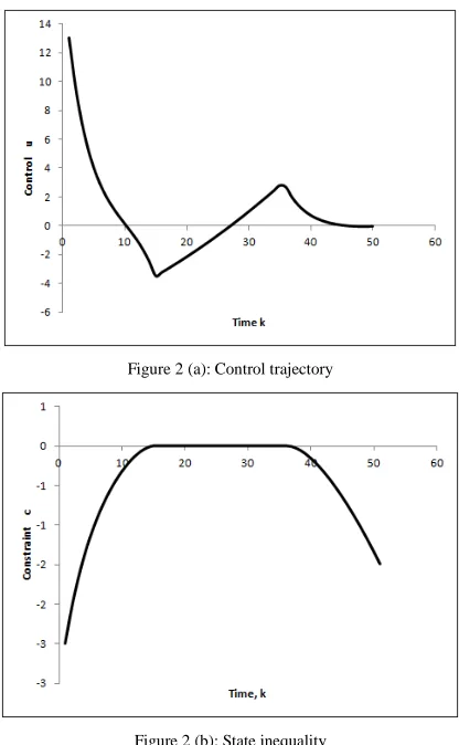
Example 2: Consider the following optimal control problem [3]:

2 2

0 1 2

( )

min ( ) ( ( )) ( ( ))

u k g u = x N + x N

1

2 2 2

1 2

0

[( ( )) ( ( )) 0.005( ( )) ]

N

k

x k x k u k

−

=

+

∑

+ +

subject to

1( 1) 1( ) 0.02 2( )

x k+ =x k + x k

x k2( + =1) 0.98x k2( )+0.02 ( )u k 2

2( ) 8(0.02 0.05) 0.5 0

x k − k− + ≤

for k=0,..., 49, with initial state

1(0) 0,

x = x2(0)= −1.

The results of control and the corresponding constraint are shown in Figures 2 (a) and 2 (b), respectively, while the minimum cost functional is g₀= 9.123153.

Figure 2 (b): State inequality

Example 3: For the state difference equations [21]

1( 1) 1( ) 0.02( ( )1 0.25)

x k+ =x k − x k +

1 2

1

25 ( )

0.01( ( ) 0.5) exp

( ) 2

x k x k

x k

 

+ +  

+

[image:4.612.75.297.258.623.2] [image:4.612.330.538.269.606.2]

(5)

26

1

0.01( ( )x k 0.25) ( )u k

− +

2( 1) 0.99 2( ) 0.005

x k+ = x k −

1 2

1

25 ( )

0.01( ( ) 0.5) exp

( ) 2

x k x k

x k

 

− +  

+

 

for k=0,..., 77,with initial condition

1(0) 0.05,

x = x₂(0)=0, the cost function

1

2 2 2

0 1 2

0

( ) 0.01 [( ( )) ( ( )) 0.1( ( )) ]

N

k

g u x k x k u k

−

=

∑

+ +

is to be minimized.

The trajectories of control and state are, respectively, shown in Figures 3 (a) and 3 (b). The minimum value of cost functional is g₀= 0.02725.

Figure 3 (b): State trajectory

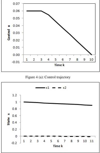
Example 4: Consider the third-order system [24]:

1( 1) 1( ) 0.01(sin( 2( ) ( 2( ) 1) 3( ))

x k+ =x k + x k + x k + x k

x k2( + =1) x k2( ) 0.01( ( )+ x k1 5+x k3( ))

x k3( + =1) x k3( )+0.01( ( )x k1 2+u k( ))

with the initial state

1(0) 1,

x = x2(0)=0, x3(0)= −1.

The aim is to find an admissible control ( )u k such that the cost function

1

2 2 2

0 1 2

0

( ) 0.01 [( ( )) ( ( )) ( ( )) ]

N

k

g u x k x k u k

−

=

∑

+ +

is minimized with the control bound 0≤u k( )≤0.06.

The results are shown in Figures 4 (a) and 4 (b) with the minimum value of cost functional g₀= 0.18299.

V. CONCLUDING REMARKS

In this paper, the NLP approach was discussed in solving optimal control problems. The control parameterization approach is applied to generalize the optimal control problem in canonical form. With this canonical formulation, the NLP model of the optimal control problem is obtained. The control variables, which are piecewise constant, are defined as decision variables in the NLP model. Their values are calculated from the gradient formulae that are derived from the canonical formulation. From the illustrative examples, the efficiency of the algorithm discussed is shown.

[image:5.612.83.291.293.595.2] [image:5.612.330.537.333.650.2]

(6)

27

ACKNOWLEDGMENT

The author would like to express his sincere thanks to anonymous reviewers for their insightful comments that helped in improving the manuscript.

REFERENCES

[1] A. E. Bryson, Dynamic Optimization, Addison-Wesley, 1999. [2] C. J. Goh and K. L. Teo, “Control parameterization: A unified

approach to optimal control problems with general constraints”, Automatica, 24, 3-18, 1988.

[3] K. L. Teo, C. J. Goh and K. H. Wong, A Unified Computational Approach to Optimal Control Problems, Longman Scientific and Technical, Essex, 1991.

[4] R. Loxton, K. L. Teo and V. Rehbock, “Computational method for a class of switched system optimal control problems”, IEEE Transactions on Automatic Control, 54, 2455-2460, 2009.

[5] R. Loxton, K. L. Teo, V. Rehbock and K. F. C. Yiu, “Optimal control problems with a continuous inequality constraint on the state and the control”, Automatica, 45, 2250-2257, 2009.

[6] Q. Lin, R. Loxton, K. L. Teo and Y. H. Wu, “A new computational method for a class of free terminal time optimal control problems”, Pacific Journal of Optimization, 7, 63-81, 2011.

[7] R. Loxton, Q. Lin, V. Rehbock and K. L. Teo, “Control parameterization for optimal control problems with continuous inequality constraints: new convergence results”, Numerical Algebra, Control and Optimization, 2, 571-599, 2012.

[8] C. R. Hargraves and S. W. Paris "Direct Trajectory Optimization Using Nonlinear Programming and Collocation", Journal of Guidance, Control, and Dynamics, 10 (4), 338–342, 1987.

[9] P. F. Gath and K. H. Well, "Trajectory Optimization Using a Combination of Direct Multiple Shooting and Collocation", AIAA Guidance, Navigation, and Control Conference, 6–9 August 2001, Montréal, Québec, Canada.

[10] J. T. Betts, Practical Methods for Optimal Control Using Nonlinear Programming, SIAM, 2001.

[11] V. M. Becerra, (2010). "Solving complex optimal control problems at no cost with PSOPT". Proc. IEEE Multi-conference on Systems and Control, September 7-10, 2010, Yokohama, Japan, 1391-1396. [12] V. M. Becerra and P. D. Roberts, “Dynamic integrated system

optimization and parameter estimation for discrete time optimal

control of nonlinear systems”, International Journal of Control, 63, 257-281, 1996.

[13] V. M. Becerra and P. D. Roberts, “Application of a novel optimal control algorithm to a benchmark fed-batch fermentation process”, Trans. Inst. Measurement Control, 20, 11-18, 1998.

[14] P. D. Roberts and V. M. Becerra, “Optimal control of a class of discrete-continuous non-linear systems decomposition and hierarchical structure”, Automatica, 37, 1757-1769, 2001.

[15] Y. Zhang and S. Y. Li, “DISOPE distributed model predictive control of cascade systems with network communication”, Journal of Control Theory and Applications, 2, 131-138, 2005.

[16] S. L. Kek, K. L. Teo and M. I. A. Aziz, “An integrated optimal control algorithm for discrete-time nonlinear stochastic system”, International Journal of Control, 83, 2536-2545, 2010.

[17] S. L. Kek, K. L. Teo, M. I. A. Aziz, “Filtering solution of nonlinear stochastic optimal control problem in discrete-time with model-reality differences”, Numerical Algebra, Control and Optimization, 2, 207-222, 2012.

[18] S. L. Kek, M. I. A. Aziz, K. L. Teo and R. Ahmad, “An iterative algorithm based on model-reality differences for discrete-time nonlinear stochastic optimal control problems”, Numerical Algebra, Control and Optimization, 3, 109-125, 2013.

[19] A. E. Bryson and Y. C. Ho, Applied optimal control, Washington, DC: Hemisphere, 1995.

[20] F. L. Lewis and V. L. Syrmos, Optimal Control, 2nd Ed., John Wiley & Sons 1995.

[21] D. E. Kirk, Optimal Control Theory: An Introduction, Mineola, NY: Dover Publications, 2004.

[22] R. E. Bellman, Dynamic Programming, Princeton University Press, Princeton, NJ, 1957.

[23] L. S. Pontryagin, V. G. Boltyanskii, R. V. Gamkrelidze and E. F. Mishchenko, The Mathematical Theory of Optimal Processes (Russian), English translation: Interscience, 1962.