Studies on the application of the alpha stable distribution in economics

by

John C. Frain

Submitted to the Department of Economics

in fulfilment of the requirements for the degree of

Doctor of Philosophy

at the

University;

b. is entirely my own work; and

c. I agree that the Library may lend or copy the thesis upon request. This permission covers only single copies for study purposes, subject to nor-mal conditions of acknowledgement.

sense in which a bubble and a bust can not occur in the usual econometric models.

These models, almost always, depend on the normal or Gaussian distribution. Yet

when one looks at data for asset prices the number and size of extreme losses and

gains are orders of magnitude greater than a normal distribution would predict. The

very existence of these extreme values must lead one to question the validity of the

normality assumption and to look for an alternative.

From time to time several alternatives have been proposed. A common

pro-posal is to use mixtures of normal distributions. The simplest such solution is to

have a mixture of two normal distributions — the first, with low volatility,

repre-sents the fundamental state with no bubble and the second, with high volatility, the

bubble. The price of the asset in question is seen as switching from one state to

the other with the switching being determined by some form of deterministic or

stochastic process. Other solutions involve what are, in effect, infinite mixtures of

normal distributions. Chief amongst these are the various GARCH proceses and the

t-distribution. Various other “fat-tailed” distributions have been proposed but these have not received universal acceptance and probably never will. While such

distribu-tions often fit the data well, We have not seen any convincing theoretical arguments

why they should.

The purpose of this thesis is to examine the use of the α-stable distribution in this context and to determine some of the consequences of its use. The α-stable distribution is a generalisation of the normal distribution. It was first proposed as

a distribution for asset returns and commodity prices by Mandelbrot in the early

1960s. It attracted a lot of attention up to the early 1970s and then interest faded.

There were two reasons for the waning interest. First the advances made at the time

in portfolio and option pricing theory were dependent on the normal distribution. At

the time almost all of this work could not have been replicated without the normality

assumption. Secondly for actual application the computer power available at the

α-anα-stable distribution. OLS estimates are not optimum. The maximum likelihood estimator of the regression coefficients is a form of robust estimator that gives less

weight to extreme observations. The theory is applied to the estimation of day

of week effects in the equity indices. The methodology is feasible and there are

sufficient differences in the results to justify the use of the new methodology when

sufficient data are available and “fat tails” are suspected. The results support the

conclusion that day of week effects no longer exist.

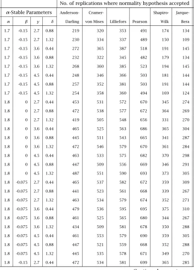
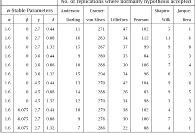
The second study is a simulation exercise to assess the power of normality tests

when the alternative is anα-stable distribution. Such tests are sometimes applied to monthly equity returns and when normality can not be rejected it is concluded

that the data can not be non-normalα-stable. We show that the power of these test is often so poor that these conclusions can not be sustained.

The third study concerns the use of the α-stable distribution in the measure-ment of Value at Risk (VaR). We find that a static α-stable distribution gives good measures of VaR at conventional levels for the equity indices examined. The α-stable distribution and a GARCH process with α-stable innovations can give very good measures of VaR.

We may draw two types of conclusion from the studies:

1. The use of theα-stable distribution is feasible in many situations. In the situa-tions examined here it appears to give better results than traditional methods

that rely on the normal distribution. It can only be used when there is a large

sample of data such as is available in the daily equity return series considered

here.

2. From a policy viewpoint there are two consequences of this analysis:

progress along the way.

First I should recall my debt to the staff of the mathematics, mathematical

physics and economics Departments in UCD where, what seems a long time ago,

I received my bachelors and masters degrees in Mathematical Science and a masters

degree in Economic Science. The training provided there has been of great

assis-tance in my career. I had considerable intellectual stimulation during the twenty

plus years before “retirement” that I worked in the economics department of the

Central Bank of Ireland. I must thank my ex-colleagues there for their

encourage-ment when I announced my intention to “retire” and do a Ph. D. We continue to keep

in touch and discuss the way in which my research may have implications for the

work of the Central Bank. I must thank Professors Frances Ruane and Alan Matthews

for their help in easing the transition from central banking to academia.

I must thank my supervisor Professor Antoin Murphy who provided

encourage-ment and guidance and ensured that the content of my thesis retained its relevance

to the real world. I regard Michael J Harrison as a true friend. He has read the

orig-inal papers that form the basis of the thesis and has provided detailed comments.

These comments and our frequent discussions and coffees were of great assistance

and encouragement to me. I thank him for his attention to detail, enthusiasm,

un-derstanding and friendship.

The economics department in Trinity College provided excellent research

facili-ties. I must thank the administrative staff, the academic staff and my fellow

post-graduate students for the excellent work atmosphere in the department.

I must also thank those who provided comments at my presentations at the IEA

annual conferences in April 2006 in Bunclody, April 2007 in Bunclody and April

2008 in Westport, at the June 2006 INFINITI conference in Dublin, at a MACSI

semi-nar in the University of Limerick in March 2007, at a Semisemi-nar in the Kemmy Business

1 Introduction 1

1.1 Preview . . . 1

1.2 Postscript . . . 10

2 Theα-stable Distribution and Equity Returns 13

2.1 Introduction . . . 13

2.2 Theα-stable Distribution . . . 23 2.3 Comparison of fit of Normal and α-stable Distributions to Returns on

Equity Indices . . . 26

2.4 Summary and Conclusions . . . 31

3 Theα-stable Distribution and Regression 43

3.1 Introduction . . . 43

3.2 Regression with Non-normalα-stable Errors . . . 46 3.3 Maximum Likelihood Estimates of Day of Week Effects with α-stable

Errors . . . 52

3.4 Summary and Conclusions . . . 61

4.2.7 Jarque-Bera Test . . . 70

4.3 Results . . . 72

4.3.1 Discussion of Results . . . 73

4.3.2 Application of tests to monthly Total Return Equity Indices . . . . 74

4.4 Summary and Conclusions . . . 74

4.5 Appendix – Tables of Detailed Results . . . 79

5 VaR and theα-stable Distribution 117 5.1 Introduction . . . 117

5.2 Value at Risk (VaR) . . . 119

5.3 Empirical Results . . . 125

5.3.1 VaR Estimates . . . 126

5.3.2 Exceedances of VaR Estimates . . . 130

5.4 Conclusions . . . 140

5.5 Appendices . . . 142

5.5.1 Maximum Likelihood estimates ofα-stable parameters . . . 142

5.5.2 GARCH estimates . . . 142

5.5.3 α-stable GARCH Estimates and VaR . . . 157

5.5.4 Data and Software . . . 160

A α-stable Distribution 161 A.1 Central Limit Theorems . . . 161

A.2 Theα-stable Distribution . . . 164

A.3 A Generalised Central Limit Theorem . . . 168

A.4 Some properties ofα-stable distributions . . . 174

A.5 Domains of Attraction . . . 175

2.1 Summary Statistics for Equity Total Return Indices and their Fit to a

Normal Distribution . . . 28

2.2 Estimates of Parameters of α-stable distributions of Equity Total Re-turn Indices (complete period) . . . 29

3.1 Summary Statistics Equity Total Return Indices and their Fit to Normal

andα-stable Distributions . . . 53

3.2 OLS Estimates of Day of Week Effects in Returns on Equity Indices . . . . 54

3.3 α-stable Estimates of Day of Week Effects in Returns on Equity Indices . 55 3.4 Summary Statistics Returns on DAX30 and their Fit to Normal and

α-stable Distributions for Three Sub-periods . . . 56

3.5 OLS Estimates of Day of Week Effects in Returns on DAX30 Index in

Three Sub-periods . . . 57

3.6 Maximum Likelihood α-stable Estimates of Day of Week Effects in Re-turns on DAX30 in Three Sub-periods. . . 58

4.1 Critical Values of Jarque-Bera Test of Normality . . . 71

Replications) . . . 86

4.7 Simulation of 5% Normality Tests onα-stable Samples of Size 200 (1000 Replications) . . . 89

4.8 Simulation of 1% Normality Tests onα-stable Samples of Size 50 (1000 Replications) . . . 92

4.9 Simulation of 1% Normality Tests onα-stable Samples of Size 100 (1000 Replications) . . . 96

4.10 Simulation of 1% Normality Tests onα-stable Samples of Size 200 (1000 Replications) . . . 99

4.11 Simulation of 10% Normality Tests onα-stable Samples of Size 50 (1000 Replications) . . . 102

4.12 Simulation of 10% Normality Tests on α-stable Samples of Size 100 (1000 Replications) . . . 105

4.13 Simulation of 10% Normality Tests on α-stable Samples of Size 200 (1000 Replications) . . . 109

4.14 Simulation of Normality Tests on a Normal Distribution (1000

replica-tions) . . . 112

5.1 10% VaR for each Equity Index forα-stable, Normal andt- distributions 127

5.2 5% VaR for each Equity Index forα-stable, Normal andt- distributions 128

5.3 1% VaR for each Equity Index forα-stable, Normal andt- distributions . 128 5.4 0.5% VaR for each Equity Index forα-stable, Normal andt- distributions 128

5.5 0.1% VaR for each Equity Index forα-stable, Normal andt- distributions 129

5.6 % Exceedances for 10% VaR for each Equity Index for Normal, Normal

GARCH,t,tGARCH,α-stable andα-stable GARCH . . . 131

Indices (complete period) . . . 143

5.13 Estimated ARMA(p,q) GARCH(1,1), Normal Innovations (CAC40) . . . 145

5.14 Estimated ARMA(p,q) GARCH(1,1),tInnovations (CAC40) . . . 146

5.15 Estimated ARMA(p,q) GARCH(1,1) Normal Innovations (DAX 30) . . . 147

5.16 Estimated ARMA(p,q) GARCH(1,1)tInnovations (DAX 30) . . . 148

5.17 Estimated ARMA(p,q) GARCH(1,1), Normal Innovations (FTSE100) . . . . 149

5.18 Estimated ARMA(p,q) GARCH(1,1)tInnovations (FTSE100) . . . 150

5.19 Estimated ARMA(p,q) GARCH(1,1), Normal Innovations (ISEQ) . . . 151

5.20 Estimated ARMA(p,q) GARCH(1,1)tInnovations (ISEQ) . . . 152

5.21 Estimated ARMA(p,q) GARCH(1,1), Normal Innovations (S&P500) . . . 153

5.22 Estimated ARMA(p,q) GARCH(1,1)tinnovations (S&P500) . . . 154

5.23 Estimated ARMA(p,q) GARCH(1,1), Normal Innovations (Dow Jones Com-posite) . . . 155

5.24 Estimated ARMA(p,q) GARCH(1,1),tInnovations (Dow Jones Composite) 156 5.25 Estimated Parameters ofα-stable GARCH Loss Distributions . . . 158

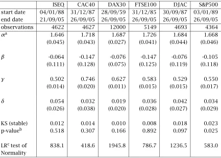
2.1 Normal QQ Plot (ISEQ returns) with 95% Limits . . . 34

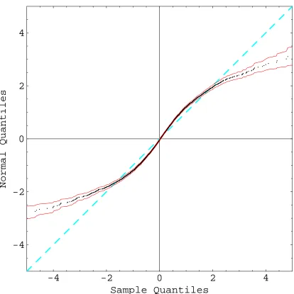
2.2 Normal QQ Plot (FTSE100 returns) with 95% Limits . . . 35

2.3 Normal QQ Plot (CAC40, DAX30, Dow Composite and S&P100 returns)

with 95% Limits . . . 36

2.4 Stable QQ Plot (ISEQ returns) with 95% Limits . . . 37

2.5 Stable QQ Plot (FTSE100 returns) with 95% Limits . . . 38

2.6 Stable QQ Plot (CAC40, DAX30, Dow Composite and S&P100 returns)

with 95% Limits . . . 39

2.7 Recursive Estimates of the Variance of Returns on Total Return Equity

Indices . . . 40

2.8 Six Simulations of the Recursive Estimation of the Variance of an α-stable Process withα₌1.7 . . . 41

3.1 Comparison of Implied Weights in GLS Equivalent of Maximum

Likeli-hood Estimates of Regression Coefficient when Disturbances are

Dis-tributed as Symmetricαstable Variates . . . 49 3.2 Comparison of Implied Weights in GLS Equivalent of Maximum

5.2 Losses on S&P 500 and 1% VaR Based on anα-stable GARCH Process . . 138

5.3 5% and 1% Static and Dynamic VaR of Losses on S&P 500 . . . 141

A.1 Normal,α-stable (α=1.5)and Cauchy Distributions . . . 169

A.2 Tails of Normal,α-stable (α₌1.5) and Cauchy Distributions . . . 170

A.3 α-stable Distribution,α₌1.5,βvarious . . . 171

Introduction

1.1

Preview

The use of the normal distribution is ubiquitous in statistical analysis in all branches of science. Ever since the days of Bernoulli (1654-1705), De Moivre (1667–1743), Laplace (1749–1827) and Gauss (1777-1855) it has been recog-nised that, subject to certain fairly unrestrictive conditions, any datum, that is the result of the aggregation of many individual data, has an approximate normal distribution. The return1 on many assets is the result of agents pro-cessing many items of information. It may be argued that the accumulation of such information is the equivalent of many shocks to returns and the result is a normal distribution of returns.

1_{Throughout this thesis the return on an asset is measured as 100 times the log}

differ-ence of the asset price (including dividends). Thus ifPt₋1andPtare the prices of the asset

in periodst₋1 andt, respectively, andDtthe dividend paid in periodt the returnRtpaid

on the asset in periodtgiven by

of $613 billion, in excess of $150 billion bond debt, and assets worth $639. On the same day Merrill Lynch agreed to sell itself to Bank of America for $50 billion,3 _{a third of its 52 week high. The shares of AIG fell from a 52} week high of $70.13 on 9 October, 2007 to a low of $1.25 on 16 September, 2008 when the Federal Reserve Board announced a loan of $85 billion, under terms and conditions4 _{that were designed to protect the interests of the U.S.} government and taxpayers. The Federal takeover of Fannie Mae and Freddie Mac 5 _{on 7 September, 2008, could be the most expensive support program} undertaken by the federal government. The plan commits the government to provide as much as $100 billion to each company to backstop any shortfalls in capital. It enables the Treasury to ultimately buy the companies outright at little cost. It also eliminates dividend payments while protecting the prin-cipal and interest payments on the debt, now held by foreign central banks, financial institutions, pension funds and others.

These events have been described6_{as once a century events. The use of the} term “once a century” probably implies that the user thinks that the events are very rare and that he does not have a good measure of how likely such events are. We would be certain that all of these companies had state of the art risk management systems. It is also likely that the use or interpretation of these systems depended, to some extent, on the normal distribution. With the benefit of hindsight, the problems arising from sub-prime mortgages, the con-sequent credit shortages and the confidence deficit were the cause of these

2_{http://www.marketwatch.com/news/story/story.aspx?guid={2FE5AC05-597A-4E71-A2D5-9B9FCC290520}&siteid=rss}

MarketWatch, 15 September 2008.

3 _{http://www.ft.com/cms/s/2/d285ebc8-82ff-11dd-907e-000077b07658.html,}

Financial Times, 16 September, 2008.

4 _{http://www.federalreserve.gov/newsevents/press/other/20080916a.htm,}

ity of such extreme events provided by the normal distribution are wrong by several orders of magnitude. A similar conclusion is reached if we apply the normal distribution to a measure of risk used by LTCM.7 _{The resulting} prob-ability is so small that the LTCM crash should not have occurred once in the entire life of the universe. The use of the normal distribution in cases such as these is leading to a gross underestimation of the risk of a large loss.

The problems arising from the use of the normal distribution are con-firmed when we look at extreme losses on equity indices. A standard mea-sure of process quality control initiated by Motorola is known as six sigma. Basically, the idea is that the standard deviation of the process is controlled so that a defective item occurs when some quality measurement is six sigma (standard deviations) below the average of the measure. In such cases, using a normal distribution suggests that such events have a probability of less than one in a billion of occurring.8 _{The six sigma theory allows for a drift in the} process and, by convention, calculates the probability as if it were 4.5 stan-dard deviations with a probability of about one in three hundred thousand. If we consider the daily loss on an equity index a six sigma event might occur on average once every 4,000,000 years (or once every 1,200 years if we use the 4.5 rule to determine the probability). These events are much rarer than the “once in a century” events we mentioned earlier. We can apply these concepts to daily returns on the FTSE100 total return price index, which is available since 31 December 1985. The six sigma for this index is 6.2%. On 19 Oc-tober 1987, 20 OcOc-tober 1987 and 26 OcOc-tober 1987 losses on the index were 11.2%, 12.2% and 6.3%, respectively. Thus there have been three six sigma events since the end of 1985 despite the fact that such events are practically

7_{See Footnote 5 on page 120}

implemen-losses. Using a normal distribution we expect a loss of greater than 4 standard deviations to occur once every 126 years. Additional losses on the FTSE100 total return index, greater than 4 standard deviations, were recorded on 11 occasions – 22 October 1987 (5.8%), 30 November 1987 (4.4%), 11 September 2001 (5.9%), 15 July 2002 (5.6%), 19 July 2002 (4.7%), 22 July 2002 (5.1%), 1 August 2002 (4.9%), 30 September 2002 (4.9%), 12 March 2003 (4.6%) and 21 January 2008 (5.6%). We must conclude that we have been very unlucky or that there is a problem with the fit of normal distribution to returns on the FTSE100. We conclude that the problem is the fit of the normal distribution to the data.

in finance. The evidence is so strong that one must conclude that the normal distribution should not be used in evaluating risk. It is not sufficient to say that these events are once off events that could not have been foreseen. The purpose of a risk management system is to get a measure of the possibility of the range of all possible changes including the very unlikely ones that may be a bit more likely than people think.

This failure of the normal distribution has considerable consequences for the conduct of business in the world of finance and in particular for the as-sessment of risk there. Any methods based on the normal distribution will underestimate risk. Various solutions have been proposed and none appears to have been universally accepted. The solution examined here is the replace-ment of the normal distribution by the α-stable family of distributions. As we shall show in Chapter 5, this distribution produces good estimates of the probability of extreme events in the equity indices considered. The use of theα-stable distribution demands considerable computational resources but these can be met in the cases considered here. As computer facilities become even more powerful it will be possible to achieve more.

treme value theory. Such procedures use the tails of the empirical distribution to make inferences about extreme values. This provides valuable results in many fields of application including insurance, hydrology, material and life sciences and finance. Here we are more interested in the properties of the entire return series.

We examine the empirical fit of theα-stable distribution to six daily total return indices (ISEQ, CAC40, DAX30, FTSE100, Dow Jones Composite (DJAC) and S&P500). We find that the fit is good. We conclude that there are good theoretical and empirical reasons to use α-stable distributions in modelling asset returns.

Our main concern is with the unconditional distribution of returns. Apart from some material on Value at Risk in Chapter 5, we do not examine the conditional distribution of returns. Any statistical analysis of equity returns is a compromise. If we use a long series, we are likely to encounter problems of non-stationarity. If we use a short period, estimates may not be sufficiently precise. In certain circumstances temporal dependencies may reduce the ef-fective size of the sample and bias estimates based on shorter samples. These problems will imply that the fit of the data is not always as good as one might expect. Apart from the DAX30, for which data are available from September 1959, the estimates in Chapter 2 are based on periods from the late 1980s up to September 2005. In Chapter 5 the sample period is extended to January 2008 and includes some of the recent turbulence on the equity markets. The estimated parameters for the extended period are not significantly different from those for the shorter period.

regres-extension of the maximum likelihood method, for symmetric α-stable dis-tributions, given in McCulloch (1998) to general α-stable distributions. The method is a form of robust estimation of the coefficients, where less weight is given to extreme observations. These weights are determined by theαand β parameters of the α-stable distribution. The methodology is then applied to the estimation of day of week effects in returns on the equity indices listed above and on the Dow Jones Industrial Average for the period covered by Gib-bons and Hess (1981), in a classic examination of such effects11_{. The results} are compared to those obtained using standard OLS and asymptotic normal theory. We find:

1. Standard errors of coefficients are somewhat smaller using theα-stable methodology.

2. We repeat the analysis of Gibbons and Hess (1981) using returns on the Dow Jones Industrial Average rather than the indices that they use. Our results are similar to theirs, rejecting the hypothesis of no day of the week effects. Our OLS estimates agrees with Gibbons and Hess (1981) in finding that returns on Monday are negative and significantly less than average and that returns are higher than average on Wednesday and Friday. The results of our α-stable analysis are similar except that we do not find higher than average returns on Wednesday.

3. For the ISEQ, CAC40, FTSE100 and DJAC there are no significant day of week effects in either the α-stable or OLS normal analyses. The esti-mates are based on the data covering the period from the late 1980s to September 2005.

compared to the starting dates of late 1980s for the other series. For the entire period both methods indicate significant day of week effects. The normal distribution indicates significantly higher returns on Wednes-days and FriWednes-days and lower on MonWednes-days. The α-stable results only in-dicate higher returns on Thursdays. Theseα-stable results may reflect the timing of Bundesbank/European Central Bank announcements. 6. Conventional wisdom would indicate that a weekend effect (high returns

on Fridays and low on Mondays) did exist at some stage but that these effect have now been arbitraged away. To look at this effect the DAX30 data were divided into three periods, September 1959 to January 1975, January 1975 to May 1990 and May 1990 to September 2005. Both methodologies indicate weekend effects in the first two periods (slightly stronger in the first) and no effects in the last period, confirming the conventional wisdom that these effects have been arbitrated away. There is sufficient evidence here to justify the examination of the robustness of Ordinary Least Squares coefficient estimates when fat-tails are suspected and sufficient data are available

the models used to measure VaR have an explicit or implicit underlying as-sumption of normality either in the estimation or scaling of the VaR estimate. Given the heavy tails in returns such an assumption is questionable.

Volatility in financial markets is a matter of considerable concern to finan-cial institutions and their supervisors. Already it is clear that this volatility has had an adverse effect on the real economy. Many measures of risk that are used today do not take full account of the kind of extreme changes in asset prices that have been observed. Chapter 5 finds that the Value at Risk measure of risk can be improved by the use of an α-stable distribution in place of more conventional measures. The chapter describes the use of this measure and implements it for six total return equity portfolios. We find that α-stable based measures can be calculated, in the cases examined, and that, as explained there, they are better measures of risk than conventional mea-sures. They are a useful tool for the risk manager and the financial regulator. If the greater probability of extreme losses as calculated from anα-stable dis-tribution had been recognised, the current market volatility, would not have surprised so many people. The recognition of this greater risk might have prevented some of the riskier ventures that have added to the depth of the current crisis.

Appendix A is a summary or the theory ofα-stable distributions. It gathers together and gives a uniform presentation of material that was included in the individual working papers on which this thesis is based.

ber/October 2008) period of extreme market volatility. Given our time con-straints, it is not feasible to extend our analysis to include this period. How-ever, I feel that I should set this analysis in context with the current situation, even though this involves duplicating some material presented elsewhere.

Our initial intention was to research bubbles and busts in asset markets. Our aim was to concentrate on equity indices where good data are readily available. Very soon we realised that the usual kind of econometric models could not account for the many extreme changes in asset prices that have occurred both over the last century and in more recent times. If the usual normal distribution is used it under-estimates the probability of such changes by many orders of magnitude.

We already had some knowledge of the α-stable distribution and decided to look at it as a probability distribution that might provide a better measure of the probability of these extreme events. Both theory and measurement confirmed that it did. The distribution, to the extent described in Chapter 5, overestimates the number of extreme movements. If the recent turbulence is taken into account the number of extreme events in the sample will increase and the fit to theα-stable distribution should be improved.

If returns follow anα-stable distribution our understanding of the current situation may be clarified. The following points are of particular importance:

was based on or interpreted using a normal distribution. However we would assume that the normal distribution played a significant part in their decisions. The implication of the α-stable assumption is that risk is usually underestimated and therefore mispriced.

• Regulators and Financial Institutions relying on the Normal distribution to set prudential ratios may have set these at too low a level. Measures of risk set at a time of low volatility may need to be increased during a period of high volatility. In periods of low volatility these limits are often not binding (see Masschelein (2007)). The implication here is that as these may involve the normal distribution they may be set to low. In a period of high volatility they will again be underestimated but they are more likely to be binding as the institution tries to contract to meet the new increased capital requirement. Such a contraction will tend to amplify any credit cycle. A change to a more realistic long-term measure of Value at Risk based to some extent on theα-stable distribution would be considerably larger than the current measure and might be binding in periods of low and high volatility. At least it would not add to the amplitude of the credit cycle. Some of the more risky investments might also have been avoided.

The

α

-stable Distribution and Equity Returns

2.1

Introduction

In this section we give a summary outline of the introduction of stochastic processes as models of asset prices paying particular attention to Brownian motion and α-stable processes. The remainder of the Chapter may be sum-marised as follows.

Section 2.2 gives a brief introduction to theα-stable distribution and should be read in conjunction with Appendix A

Section 2.3 analyses six daily total return indices (ISEQ, CAC40, DAX30, FTSE100, Dow Jones Composite and S&P500). Normal and α-stable distribu-tions are fitted to the daily returns on these indices and the fits are compared. In all cases tests of the fit reject the normal distribution. The normal

distribu-1_{This Chapter is based on a paper presented at:}

QQ-plots further show the superior fit of theα-stable distribution. Section 2.4 summarises the Chapter.

Louis Jean-Baptiste Alphonse Bachelier is often regarded as the father of the modern theory of mathematical finance. His Ph. D. thesis (Bachelier (1900a)):2

• Described the institutional details of trading on the French Exchange.

• Defines Brownian motion and argues that stock prices follow a Brow-nian motion He argues that the increments in stock prices are serially independent, follow a normal distribution and have zero expected value. (The continuity requirement for Brownian motion is implicit).

• Assumes the Markov property i.e. the next price depends only on the current price, regardless of history.

• Provides a method of valuing futures and options on that exchange.

The thesis anticipates much of the developments in stochastic calculus that were refined in the twentieth century and which were used in finance, physics and various other fields. Brownian motion is named after the English botanist Robert Brown whose research dates to the 1820s. It was rediscovered, inde-pendently, by Einstein (1905) in a paper that contributed to the acceptance of the atomic theory of matter. It was given a rigorous mathematical foun-dation by Wiener in the 1920s and is now known as Brownian motion or the Wiener Process. In recognition of Bachelier’s contribution Feller (1971, p. 99), refers to Brownian motion as Brownian motion or Wiener-Bachelier Process.

2 _{It perhaps a little inaccurate to refer here to his Ph.D. thesis as the paper in question}

probability and mathematical finance. Evidence of the importance of the the-sis is provided by the fact that the original is still in print as Bachelier (1900b), on the internet3 _{and in two English translations (in Cootner (1964b) and in} Davis and Etheridge (2006)).

Bachelier’s analysis of stock prices is based on the normality of the actual stock prices. He assumes that the change in price is independent of the level Bachelier (1900a, p. 35) and that the price follows a Brownian motion. Today we would assume that the logarithm of the price follows a Brownian motion. He recognises the possible problem and argues that the approximation is jus-tified as the distribution of the price of the stock being examined is close to symmetric and that the probability of price being negative is so small that it is effectively zero. As he is dealing with the distribution of future spot prices and the valuation of close to the money options on short dated low volatility high-liquidity government stock, this approximation would have been satis-factory.

It is perhaps somewhat surprising that he and the discussants were some-what surprised at this result. One discussant (K. S. Rao) demonstrated that it is possible to have zero correlations even when a time-series is completely deterministic. The paper or the discussants did not mention that zero correla-tion and independence are equivalent only when the distribucorrela-tions are normal. Perhaps there was an implied assumption that the distributions were asymp-totically normal or could, for practical purposes, be taken as normal. Apart from this article there appears to have been little attention devoted to the distribution of returns until the 1960s (see, for example, the introduction to Cootner (1964b)).

The purpose of Osborne (1959)5_{is to show that the logarithms of common} stock prices follow a Brownian motion. It would appear that Osborne was not familiar with Bachelier’s work. Alexander (1961) includes Bachelier (1900a) in his references. He re-analyses the data used in Kendall (1953) and verifies and amends the results found there. His analysis uses the logarithms of the variables rather than their levels.

During the 1960s and the early 1970s the normality assumption underly-ing various asset returns was questioned by, in particular, Mandelbrot (1962, 1963, 1967, 1997), (see also Mandelbrot and Hudson (2004)) and Fama (1964, 1965a, 1976). The mathematicians had already worked on processes that were a generalisation of Brownian motion, which maintained the tion of stationary independent increments, dropped the normality assump-tion, and imposed certain continuity restrictions6 _{and are now known as Lévy}

5 _{M. F. M. Osborne was a physicist working with at the Naval Research Centre of the}

followed by the increments of a Brownian motion.

Mandelbrot examined the variation of prices of cotton (1816-1940), wheat (1883-1936), railroad stock (1857-1936) and interest and exchange rates (sim-ilar periods) and found a larger number of extreme values than could be jus-tified by the assumption of a normal distribution. Fama examined the distri-bution of daily returns for the 30 stocks in the Dow Jones Industrial Average in a period from about the end of 1957 to 26 September 1962. These papers offered support for the hypothesis that returns followed an α-stable7 _rather than a normal process. Anα-stable distribution may be thought of as a gen-eralisation of the normal distribution where the gengen-eralisation allows greater concentration close to the mean, more extreme values and possible skewness. We will see that the normal distribution is anα-stable with restricted param-eter values. This pioneering work of Mandelbrot and Fama and others was extended over the next few years in areas such as:

Fama (1971) CAPM and α-stable processes — see appendix Section A.6 of

this thesis.

Blattberg and Sargent (1971) Regression with non-gaussian stable disturbances

— see McCulloch (1998) and Chapter 3 of this thesis for a more modern treatment based on Maximum likelihood.

DuMouchel (1971, 1973, 1975) Maximum Likelihood Estimation of the

pa-rameters of anα-stable processes.

Chambers et al. (1976) Simulation ofα-stable random variables.

Kanter (1976), Logan et al. (1973) Properties ofα-stable distributions.

7_{There is a certain confusion in the literature about the name to be given to this family of}

normal distribution had contributed, or was about to contribute, to major breakthroughs in empirical and theoretical finance. The success and impor-tance of this work can be gauged by the fact that Nobel prizes have since been awarded to Markovich, Millar, Sharpe, Merton and Scholes for their work on portfolio allocation, Capital Asset Pricing model, Option Pricing and other contributions to the theory of investment. This normal distribution played an important part in these developments. The fear was, quoting Cootner (1964a), page 418.

Mandelbrot, like Prime Minister Churchill before him, promises us

not utopia but blood, sweat, toil and tears. If he is right, almost all of

our statistical tools are obsolete — least squares, spectral analysis,

workable maximum-likelihood solutions, all our established sample

theory, closed distribution functions. Almost without exception, past

econometric work is meaningless....

ingα-stable distributions were ingenious and should be evaluated in the con-text of the facilities available at the time. The arguments advanced against the suitability of α-stable distributions also need to be re-examined. Given the available technology at the time, both sides of the argument did as much as could have been done at the time. With today’s resources much more can be done and we would prefer not to use the empirical work done at that time to argue for or against the validity of the use of the α-stable distribution in finance. It is a pity that a some modern texts (e.g. Taylor (2005)) dismiss the α-stable distribution on the evidence of authors such as Blattberg and Gonedes (1974)10_{, Hagerman (1978) and Perry (1983)}11 _{who did not have the} use of modern technology.

The problem with Cootner’s view is that he sees models arising from the normal andα-stable distributions as totally contradictory. In the majority of

9 _{Renfro (2004) contains a comprehensive account of the development of econometric}

software.

10_{Blattberg and Gonedes (1974) give empirical arguments for the use of thet-distribution.}

The methods they use to estimate the parameters of an α-stable distribution need to be updated. While their empirical arguments are strong they do not offer any theoretical reasons why asset returns follow at-distribution rather than anα-stable.

11 _{Perry’s argument is that if returns follow an α-stable distribution estimates of the}

to effectively skip it. This will lead to a more robust estimate and one that is likely to be closer to an α-stable based estimate if such were feasible. As the peak of a normal distribution is wider than that of a stable distribution my intuition is that the use of the normal distribution may lead to conserva-tive confidence intervals, at the conventional 10% and 5% confidence levels. Given the dependence of econometrics on asymptotic results that are only approximate in small samples this may not be a disadvantage.

When, as in the analyses here, the data series are long enough they should be analysed using the best tools available. In the analysis here, using theα -stable distribution does give results that correspond more closely with reality. When conventional normal distribution based methods are used the analyst and management should be aware of the possible defects in the model. At least the results should be examined to see how robust they are with respect to the choice of distribution. Whileα-stable distributions, in general, do pro-vide a much better fit to the returns we examine here, they still give rise to considerable implementation problems both on an empirical and theoretical basis. However, as we show there is much that can be done and as computer power increases and more data become available the α-stable distribution will become easier and cheaper to use and will therefore be used more often. Economists should be aware of these results.

return index shows 6 such falls in the period from January 1989 to September 2005. The normality assumption would imply an expected period of 12,000 years. The distribution of increases shows similar discrepancies between the empirical distribution and the normal distribution.

These extreme events are the Black Swans of Taleb (2004, 2007). Accord-ing to Taleb, the cygnus atratus is a black swan which is native to Australia. Native swans in Europe are white. Prior to the discovery of the black swan in Australia a European might have assumed that all swans were white and he would have been totally surprised by the finding of a black swan. Taleb attributes the problem to invalid induction. If the distribution or returns is normal the extreme returns on equity returns are black swans. Under an α -stable distribution these black swans become a shade of gray and we should not be taken by surprise if they occur.

supervisors. It is of particular importance to those who are measuring risk using a Value at Risk system based on an assumption that returns follow a normal distribution. If the element of risk is underestimated in equity price models, which assume normality, alternative models may provide some ex-planation of the excess equity premium paradox.

The fat tails of the distribution of returns can be fit by a variety of other distributions in addition to the α-stable. It is often argued that the fat tails can be accommodated by a polynomial decay in the tails of the distribution ie the asymptotic probability density function of the extreme values of the tails is given by

fX(x, α)=cx−(1+α), forx > x0.

When 0 < α _≤ 2 we are in the realm of an α-stable distribution. Extreme value theory often leads to an estimate of αof the order of 4 for the tails of the return distribution. The t and Pareto distributions are examples of such fat tailed distributions. These do not have the scaling properties that we find desirable in return distributions. Also Weron (2001) shows that estimates of α for α-stable distributions with α taking values in the range found here, from extreme value theory, may be biased upward and often give estimates ofαgreater than 2. Appendix A gives further details.

Applications to Finance are covered in Mittnik et al. (2000)

2.2

The

α

-Stable Distribution

This section contains a brief introduction to the α-stable distribution. Ap-pendix A contains a more complete technical description and references. The α-stable distribution is a family of statistical distributions which is indexed by a parameter α which can be any positive number less than or equal to 2. When α ₌ 2 the α-stable distribution becomes a normal distribution. When α ₌ 1 the distribution becomes a Cauchy distribution. As α is decreased larger extreme values become more likely.

A second parameter, β measures the skewness of the distribution. β can take values from ₋1 to 1. When β = 0 the distribution is symmetric. A positive value of β implies that the distribution is skewed to the right (i.e. Large positive values are more likely than large negative values). Larger values ofβ imply greater positive skewness. Similarly negative values of beta imply that large negative values are more likely than large positive. It is sometimes thought that equity return distributions are negatively skewed. As the normal distribution is symmetric it can not model any skewness in the data.

The α-stable distribution requires two more parameters — a spread pa-rameter,γ, and a location parameter,δ. These are similar in interpretation to the mean, µ and standard deviation, σ, respectively, of the normal distribu-tion.

The α-stable distribution has several features that make it an attractive model of returns:

tion with this property. If we could account for possible time of day, day of week, other seasonal effects and other non-stationarities that are inherent in the return generating process we might assume that returns aggregated over time have the same distribution, up to a scale and loca-tion factor, as the original higher frequency data. Such data then must have anα-stable distribution. The normal distribution is one particular member of the family of α-stable distributions. The general α-stable distribution allows one to retain this property while allowing the data to be modelled in a more flexible manner.

4. The α-stable distribution replaces the normal distribution in what is known as the generalised central limit theorem. A non-normalα-stable distribution may be the limit distribution of sums of random variables that do not satisfy the requirements of the Lindeberg-Lévy-Feller central limit theorem. Thus where an equity or portfolio return is the result of an accumulation of shocks (news) theα-stable distribution may provide a good approximation. This argument is basically the same as that used to justify a normal distribution.

mathematical functions. Otherwise the density function must be esti-mated using numerical methods. Modern computers facilitate this pro-cess.

Table 2.1 gives summary statistics for each of the six total return indices. Each return series is given in its domestic currency and no attempt has been made to convert series to a common currency. The most notable features of these statistics are the extreme estimates of the kurtosis of returns. This is an indication of the long tails in the data. The table also estimates three statistics which function as goodness of fit tests15_{to the normal distribution.}

Jarque and Bera (JB) test The JB test is a joint test for skewness and excess

kurtosis relative to a normal distribution. Given a data sample_{xi, i= 1, . . . , N_}with mean ¯x the JB test statistic is estimated16 as follows:

ˆ σ2

= _N1

−1Σ i=N

i=1(xi−x)¯ 2, mk=

1 NΣ

i=N

i=1(xi−x)¯ k, k=2,3,. . . , b11/2=

N2

(N₋1)(N₋2) m3

ˆ

σ3 (Skewness), b21/2=

N2

(N−1)(N−2)(N−3)

(N₊1)m4₋3(N₋1)m22 ˆ

σ4 (Kurtosis),

JB₌N (b 1/2 1 )2

24 +

(b₂1/2)2 6

!

(Jarque-Bera statistic).

Under the assumption that thexiare independent identically distributed normal random variables the Jarque-Bera statistic is asymptotically χ2 with 2 degrees of freedom. In this case the statistics indicate very sig-nificant departures from a normal distribution.

Kolmogorov Smirnov (KS) test The KS test in this case compares the

When the mean and variance of the normal distribution are unknown critical values of the KS test for normality are given in Lilliefors (1967). The 1% critical values in this case are 0.014 for the FTSE100, 0.015 for the ISEQ, CAC40 and DJAC, 0.016 for the S&P500 and 0.009 for the DAX30. The values found indicate very significant departures from nor-mality.

Shapiro Wilk (SW) test The SW test is based on the correlation between x(i)

and F−1_(i/N

+1) which are the i/n quantiles of the sample and pop-ulation respectively.17 _{Again the normal hypothesis is rejected and the} conclusions following the JB and KS statistics are confirmed.

start date 04/01/88 31/12/87 28/09/59 31/12/85 30/09/87 03/01/89 end date 21/09/05 26/09/05 26/09/05 26/09/05 26/09/05 26/09/05

observations 4622 4627 12000 5149 4693 4363

mean 0.052 0.044 0.022 .041 0.038 0.043

St. dev 0.934 1.277 1.148 1.028 1.007 0.980

Skewness -0.3634 -0.124 -0.282 -0.732 -2.686 -0.198 Kurtosis 5.376 3.002 8.378 9.814 58.1964 4.282

JB testa 5690 1749 35254 21123 667907 3362

KS testb 0.065 0.054 0.062 0.055 0.074 0.063

SW testc _{0.941 0.967 NA NA 0.8689 0.956}

a _{The asymptotic distribution of the Jarque-Bera statistic is χ}2_{(2) with critical} values 5.99 and 9.21 at the 5% and 1% levels respectively.

b_{See text}

c _{The 5% critical level for the Shapiro Wilk test is .9992 for a sample of 4500. The} smaller values reported here indicate very significant departures from normal-ity.

empirical distribution relative to the normal at the centre of the distribution.

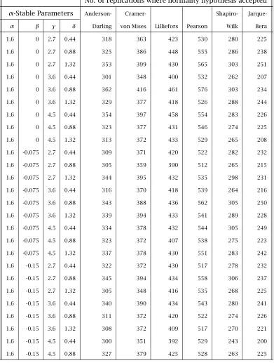
Table 2.2: Estimates of Parameters of α-stable distributions of Equity Total Re-turn Indices (complete period)

ISEQ CAC40 DAX30 FTSE100 DJAC S&P500 start date 04/01/88 31/12/87 28/09/59 31/12/85 30/09/87 03/01/89 end date 21/09/05 26/09/05 26/09/05 26/09/05 26/09/05 26/09/05

observations 4622 4627 12000 5149 4693 4364

αa _{1.646 1.718 1.687 1.726 1.684 1.668}

(0.045) (0.043) (0.027) (0.041) (0.044) (0.046)

β -0.064 -0.147 -0.076 -0.147 -0.076 -0.105

(0.111) (0.128) (0.075) (0.125) (0.119) (0.118)

γ 0.502 0.746 0.627 0.583 0.529 0.550

(0.014) (0.020) (0.011) (0.015) (0.015) (0.017)

δ 0.054 0.032 0.019 0.036 0.042 0.034

(0.026) (0.038) (0.020) (0.028) (0.027) (0.029)

KS (stable) 0.012 0.014 0.010 0.008 0.018 0.023

p-valueb _{0.518 0.307 0.166 0.892 0.097 0.025}

LRctest of 838.1 418.6 1945.8 786.7 1236.5 583.0 Normality

a _{Figures in brackets below the estimated parameters are the 95% confidence} interval half width-estimates

b_{The p-values for the KS statistic are calculated on the assumption that the} values of α, β, γ and δ are chosen independently of the sample. As the α -stable parameters are estimates the calculated p-values overestimate true sig-nificance level.

replaced by the α-stable distribution with parameters taken from Table 2.2. The fit for the European indices is good. At the extremes there is a suggestion that the tails of the empirical distribution are a little lighter than the theoreti-cal stable distribution but this is not significant. What is surprising is that the fit in the centre of the distribution is so superior to that of the normal distri-bution. The fit of the American indices to the stable distribution is again far superior to that of the normal distribution. There are some deviations in the centre of the American distribution which are not obvious in the diagrams. These are very small relative to the deviations from the normal distribution but might be the subject of further work.

If x1, x2, . . . , xn is a random sample from a non-normal α-stable distribu-tion the estimated sample variance is given by

ˆ σn2=

1 n₋1

n

X

i=1 (x2

i −x)¯ 2

the sample sizes available, this inference is not valid.

Similar simulations with one million replications do tend to show a greater tendency for variance to increase. Simulations withα₌1.2 also tend to show increasing recursive variance estimates. The increases in the recursive esti-mates of the variance are caused by the large observations that occur in the tail of the distribution. The higher peaks in the centre of the distribution (the majority of observations) tend to cause the recursive variance to fall between extreme peaks. There is some indication of a deficit of extreme observations in the recursive estimates derived from the equity index returns. This point is discussed in Chapter 5

2.4

Summary and Conclusions

In this chapter we have examined the application of the family of α-stable distributions to daily returns on six total return equity indices (ISEQ, FTSE100, DAX40, CAC30, S&P500 and the Dow Jones Composite Total Return (DJAC)).

Section 2.2 and Appendix A of the paper outline the basic probability theory underlying these processes and explain their relevance to finance.

Early support for the use of α-stable processes in economics and finance came from the writings of Mandelbrot and Fama during the 1960s and 1970s. They found that many asset returns had features typical of these processes. After an initial period of research, interest in stable processes appeared to decrease. While computation problems were probably the main cause of this decline, a further contributing factor was the major breakthroughs in finance, achieved at that time. These were largely based on the assumption of an un-derlying normal distribution. The success of this work using the normal dis-tribution can be gauged by the fact that Nobel prizes have since been awarded to Markovich, Millar, Sharpe, Merton and Scholes for their work on portfolio allocation, Capital Asset Pricing model, Option Pricing and other contribu-tions to the theory of investment. These developments have formed the ma-jor constituents of the research agenda in quantitative finance ever since. An erroneous opinion circulating at that time was that the acceptance ofα-stable distributions would invalidate not only this work but most econometric work completed up to that time. It is only in more recent years that advances in computing facilities have facilitated increased interest in α-stable processes and this trend is likely to continue.

For all six total return indices examined here,

• The normal distribution is a very poor fit to the empirical distribution of the returns on all six indices.

• Theα-stable distribution provides a good fit.

-4

-2

0

2

4

Sample Quantiles

-4

-2

0

2

4

Normal

Quantiles

-4

-2

0

2

4

6

Sample Quantiles

-4

-2

0

2

4

6

Normal

Quantiles

Normal QQ

_-

plot FTSE100

-4 -2 0 2 4 6 Sample Quantiles -4 -2 0 2 4 6 Normal Quantiles

Normal QQ_-plot Dow Jones

-4 -2 0 2 4 6

Sample Quantiles -4 -2 0 2 4 6 Normal Quantiles

Normal QQ_-plot S&P100

-4 -2 0 2 4 6

Sample Quantiles -4 -2 0 2 4 6 Normal Quantiles

Normal QQ_-plot CAC40

-4 -2 0 2 4 6

Sample Quantiles -4 -2 0 2 4 6 Normal Quantiles

Normal QQ_-plot DAX30

-4

-2

0

2

4

Sample Quantiles

-4

-2

0

2

4

Stable

Quantiles

-4

-2

0

2

4

6

Sample Quantiles

-4

-2

0

2

4

6

Stable

Quantiles

Stable QQ

_-

plot FTSE100

-4 -2 0 2 4 6 Sample Quantiles -4 -2 0 2 4 6 Stable Quantiles

Stable QQ_-plot Dow Jones

-4 -2 0 2 4 6

Sample Quantiles -4 -2 0 2 4 6 Stable Quantiles

Stable QQ_-plot S&P100

-4 -2 0 2 4 6

Sample Quantiles -4 -2 0 2 4 6 Stable Quantiles

Stable QQ_-plot CAC40

-4 -2 0 2 4 6

Sample Quantiles -4 -2 0 2 4 6 Stable Quantiles

Stable QQ_-plot DAX30

0 1000 2000 3000 4000 0.65 0.75 0.85 Index ISEQ variance

0 1000 2000 3000 4000

1.0 1.2 1.4 1.6 Index CAC40 variance

0 2000 4000 6000 8000 10000

0.8 1.2 1.6 Index DAX30 variance

0 1000 2000 3000 4000

0.65 0.75 0.85 Index FTSE100 variance

0 1000 2000 3000 4000

0.55

0.65

0.75

0.85

Index

Dow Jones Composite

variance

0 1000 2000 3000 4000

0.5 0.7 0.9 Index S&P 500 variance

0 1000 2000 3000 4000 2.8 3.2 3.6 4.0 Index variance

0 1000 2000 3000 4000

4 5 6 7 8 Index variance

0 1000 2000 3000 4000

10 20 30 40 50 Index variance

0 1000 2000 3000 4000

4 6 8 10 Index variance

0 1000 2000 3000 4000

5.0 6.0 7.0 8.0 Index variance

0 1000 2000 3000 4000

5 10 15 20 Index variance

Maximum Likelihood Estimates of Regression

Coefficients with

α

-stable Disturbances and

Day of Week effects in Total Returns on Equity Indices

3.1

Introduction

cent mathematical accounts are given in Zolotarev (1986), Samorodnitsky and Taqqu (1994), Weron (1998) and Uchaikin and Zolotarev (1999). Rachev and Mittnik (2000) surveys the use ofα-stable models in finance.

The availability of cheap powerful computer hardware has made advanced computation resources available to scientists in many fields. The resulting in-creased demand for good software has provided the incentive to produce and distribute widely software packages such as MATHEMATICA (Wolfram (2003)) and R (R Development Core Team (2008)) which have facilitated the calcula-tions in this Chapter. Programs to computeα-stable distribution and density functions are available in both of these packages — MATHEMATICA (Rimmer (2005)), Rmetrics for R (Wuertz (2007)) — or as the stand-alone program STA-BLE (Nolan (2006)). These resources allow one to examine the consequences of replacing the normal assumption with the more generalα-stable. Further advances in theory and computation facilities will facilitate this process in the coming years and the use of the α-stable distribution will become more common.

In particular, this chapter examines the consequences of α-stable distur-bances in OLS estimation. In Section 3.2 the following results are set out:

• Standard OLS estimates are consistent ifα >1 but inefficient.

• Coefficient estimates have anα-stable distribution and standard t-statistics do not have the usual distribution.

• Maximum likelihood estimators have the usual asymptotic properties. Confidence intervals and inference may be based on the usual maximum likelihood theory.

lihood. Estimates are made for six total return indices (ISEQ, CAC40, DAX30, FTSE100, Dow Jones Composite (DJAC) and S&P500) and the DJIA2 _{for the} period used in the often quoted study of these effects in Gibbons and Hess (1981). My results can be summarised as follows

-• The α-stable maximum likelihood and OLS estimates for the DJIA for the Gibbons and Hess (1981) period are almost identical to theirs.

• Data for the total return indices are only available from the late 1980s (apart from the DAX30) and there are no significant day of week effects in the total return indices in that period

• When the data for the CAC40 are split into three equal periods there are indications of day of week effects in the two early periods but they are absent in the last period.

These results are a demonstration of the shifting Monday effect reported in the literature (see Pettengill (2003) and the references there and Hansen et al. (2005)). Such results are, therefore, not sensitive to the use of the “robust” α-stable Maximum Likelihood Estimator.

yi = k

X

j=1

xijβj+εi, i=1, . . . , N, (3.1)

whereyiis an observed dependent variable, thexij are observed independent variables, βj are unknown coefficients to be estimated and εi are identically and independently distributed. Equation (3.1) may be written in matrix form as

y y

y ₌XXXβββ₊εεε, (3.2)

where

yyy =

        y1 y2 .. . yN        

, XXX=

       

x11 x12 . . . x1k x21 x22 . . . x2k

..

. ... . .. ... xN1 xN2 . . . xNk

       

, βββ=

        β1 β2 .. . βk        

, εεε=

        ε1 ε2 .. . εN         . (3.3)

The standard OLS estimator ofβββ is

ˆ β β

β_{OLS =}(XXX000XXX)−1XXX000yyy. (3.4)

Thus ˆ β β

β_OLS−βββ₌(XXX000XXX)−1_XXX000_{εεε. (3.5)}

-3. Asα_→2 the density tends to normal and the peaks vanish.

When 1 < α <2 the OLS estimates are consistent but converge at a rate of nα1−1 rather thann−

1

2 in the normal case.

DuMouchel (1971, 1973, 1975) shows that, subject to certain conditions (_∃ε > 0, α > ε, _|β_| < 1) the maximum likelihood estimates of the param-eters of an α-stable distribution have the usual asymptotic properties of a maximum likelihood estimator. They are asymptotically normal, asymptot-ically unbiased and have an asymptotic covariance matrix n−1

I(α, β, γ, δ)−1 where _I(α, β, γ, δ) is Fisher’s Information. McCulloch (1998) examines linear regression in the context ofα-stable distributions paying particular attention to the symmetric case. Here the symmetry constraint is not imposed. Assume thatεi =yi−Pkj=1xijβj isα-stable with parameters{α, β, γ,0}. If we denote theα-stable density function bys(x, α, β, γ, δ)then we may write the density function of εi as

s(εi, α, β, γ, δ)= 1 γ s

 yi−

Pk

j=1xijβj

γ , β,1,0



, (3.6)

the likelihood as

L(εεε, α, β, γ, β1, β2, . . . )₌ 1 γ

!n n_Y

i=1 s

 yi−

Pk

j=1xijβj

γ , β,1,0



, (3.7)

and the loglikelihood as

l(εεε, α, β, γ, β1, β2, . . . )₌ n

X

₋log(γ)₊log

 s

 yi−

Pk

j=1xijβj

, β,1,0

i=1 n

X

i=1

−φ0(εˆi)

ˆ εi

ˆ

εixim=0, m=1,2, . . . , k n

X

i=1

−φ0_εˆ(εˆi)

i

(yi− k

X

j=1

xijβj)xim=0, m=1,2, . . . , k

n

X

i=1

−φ0_εˆ(εˆi)

i

yixim= n

X

i=1

−φ0_εˆ(εˆi)

i k

X

j=1

xijβjxim

(3.9)

IfWWW is the diagonal matrix

W W W ₌        

−φ0(εˆ1)

ˆ

ε1 0 . . . 0

0 ₋φ0(εˆ2)

ˆ

ε2 . . . 0

..

. ... . .. ... 0 0 . . . −φ0(εˆn)

ˆ εn         , (3.10)

Using the notation in Equation (3.3) we may write Equation (3.9) in matrix format as

X X

X0WWW yyy ₌(XXX0WWW XXX)ββˆβ, (3.11)

or ifXXX0WWW XXX is not singular

ˆ β β

β₌(XXX0WWW XXX)−1_XXX0_{WWW yyy. (3.12)}

Thus the maximum likelihood regression estimator has the format of a Generalised Least Squares estimator in the presence of heteroscedasticity where the variance of the error term εi is proportional to φ

0_(εi) εi .

ef--6 -4 -2 2 4 6

residual 0.5

1.0 1.5 2.0

weight

Normal 1.6 1.2

are drawn with γ = 1/ 2. As expected the normal distribution gives equal weights to all observations. The estimator forα-stable processes gives higher weights to the centre of the distribution and extremely small weights to ex-treme values. This effect increases asαis reduced.

This result explains the results obtained by Fama and Roll (1968) who completed a Monte Carlo study of the use of truncated means as measures of location inα-stable distributions. They found:

When α ₌ 1.1 the .25 truncated4 means are still dominant for all n. For α₌ 1.3 andα₌ 1.5 the .50 truncated means are generally best, and whenα₌1.9the distributions of the.75truncated means are uniformly less disperse than those of other estimators. Finally,

when the generating process is Gaussian (α ₌ 2) the mean is the “best” estimator. Of course it is also minimum-variance, unbiased

in this case.

-6 -4 -2 2 4 6

residual

-1.0 -0.5

0.5 1.0 1.5 2.0

weight

Normal 1.6 1.2

Empirical analysis suggests that there is a recurrent low or negative return on equities from Friday to Monday. This effect is known as the weekend ef-fect. The existence of this effect would allow one to design a strategy to make excess profits and would have implications for the Efficient Markets Hypoth-esis. It is likely that if disturbances are α-stable, then the usual Ordinary Least Squares inferences may lead to spurious results. The use of α-stable disturbances and maximum likelihood will lead to more robust results.

The analysis is based on daily data for six equity indices (ISEQ, CAC40, DAX30, FTSE100, Dow Jones Composite(DJAC) and S&P500) which have been adjusted to include dividends. Thus if Pt and Dt are the price and dividend of the index in periodt the return on the index in periodt is given by

Rt =100 log

_P

t+Dt Pt−1

≈100

_P

t+Dt Pt−1 −

1

. (3.13)

We have also used returns based on the historic values of the Dow Jones Industrial Average equity price index covering the period 3 July 1962 to 28 December 1978, the period analysed in Gibbons and Hess (1981). These have not been adjusted for dividends.

Descriptive statistics and details of goodness of fit of the return series to Normal and α-stable distributions are given in Table 3.1.5 _{The goodness of} fit normality tests indicate considerable problems with the fit of a Normal distribution. Theα-stable distribution provides a better fit.

To estimate and test for day of week effects returns were regressed on five dummy variables, one for each day of the week. The presence of a day of week effect is indicated by the rejection of the hypothesis that all five regression coefficients are equal.