An Interactive Fuzzy Satisficing Method for
Multiobjective Linear Programming Problems
with Random Fuzzy Variables Using
Possibility-based Probability Model
Masatoshi Sakawa
∗,
Takeshi Matsui
,
Hideki Katagiri
Faculty of Engineering, Hiroshima University, Higashi-Hiroshima, 739-8527, Hiroshima, Japan
∗Corresponding Author: [email protected]
Copyright c⃝2014 Horizon Research Publishing All rights reserved.
Abstract
This paper formulates multiobjective linear programming problems where each coefficient of the objective functions is expressed by a random fuzzy variable. Assuming that the decision maker concerns about the probability that each of the objective function values is smaller than or equal to a certain target value, the fuzzy goals of the decision maker for the probabilities are introduced. Then, the possibility-based probability model to maximize the degrees of possibility with respect to the attained probability is considered. For solving transformed deterministic problems efficiently, particle swarm optimization for nonlinear programming problems is introduced. An interactive fuzzy satisficing method is presented for deriving a satisficing solution for a decision maker efficiently by updating the reference probability levels. An illustrative numerical example is provided to demonstrate the feasibility and efficiency of the proposed method.Keywords
Multiobjective linear programming, Random fuzzy programming, Possibility, Probability maximization, Interactive method1
Introduction
In actual decision making situations, we must often make a decision on the basis of vague information or uncertain data. For such decision making problems in-volving uncertainty, there exist two typical approaches: probability-theoretic approach [1–4] and fuzzy-theoretic one [5–7]. Stochastic programming, as an optimization method based on the probability theory, have been de-veloping in various ways including two stage problems considered by Dantzig [8] and chance constrained pro-gramming proposed by Charnes et al. [9].
In most practical situations, however, it is natural to consider that the uncertainty in real world decision mak-ing problems is often expressed by a fusion of fuzziness and randomness rather than either fuzziness or
random-ness. For handling not only the decision maker’s vague judgments in multiobjective problems but also the ran-domness of the parameters involved in the objectives and/or constraints, Sakawa and his colleagues incorpo-rated their interactive fuzzy satisficing methods for de-terministic problems [5, 10] into multiobjective stochas-tic programming problems, through the introduction of several stochastic programming models such as expec-tation optimization [11, 12], variance minimization [11], probability maximization [11, 13, 14] and fractile crite-rion optimization [11], to derive a satisficing solution for a decision maker from Pareto optimal solution sets.
In multiobjective stochastic programming problems, it is implicitly assumed that uncertain parameters or co-efficients can be expressed as random variables in prob-ability theory. This means that the realized values of random parameters under the occurrence of some event are assumed to be definitely represented with real values. However, it is natural to consider that the possible re-alized values of these random parameters are often only ambiguously known to the experts. In this case, it may be more appropriate to interpret the experts’ ambigu-ous understanding of the realized values of random pa-rameters under the occurrence of events as fuzzy num-bers. From such a point of view, a fuzzy random variable was first introduced by Kwakernaak [15], and its mathe-matical basis was constructed by Puri and Ralescu [16]. Studies on linear programming problems with fuzzy ran-dom variable coefficients, called fuzzy ranran-dom linear pro-gramming problems, were initiated by Wang and Qiao [17] and Qiao, Zhang and Wang [18] as seeking the prob-ability distribution of the optimal solution and optimal value.
method [19].
A recently published book of Sakawa et al. [20] is devoted to introducing the latest advances in the field of multiobjective optimization under both fuzziness and randomness on the basis of authors’ continuing research works. Special stress is placed on interactive deci-sion making aspects of fuzzy stochastic multiobjective programming for human-centered systems under uncer-tainty in most realistic situations when dealing with both fuzziness and randomness.
Under these circumstances, in this paper, we con-sider multiobjective linear programming problems in-volving random fuzzy variables. To deal with the formu-lated random fuzzy multiobjective linear programming problems, we assume that the decision maker concerns about the probabilities that each of the objective func-tion values is smaller than or equal to a certain target value. By considering the imprecise nature of the human judgments, we introduce the fuzzy goals of the decision maker for the probabilities. Assuming that the deci-sion maker is willing to maximize the degrees of possi-bility with respect to the attained probapossi-bility, we con-sider the possibility-based probability model for random fuzzy multiobjective linear programming problems. For solving transformed deterministic problems efficiently, particle swarm optimization for nonlinear programming problems [22] is introduced. Then, we present an in-teractive fuzzy satisficing method to derive a satisficing solution for the decision maker by updating the reference possibility levels. An illustrative numerical example is provided to demonstrate the feasibility and efficiency of the proposed method.
2
Random fuzzy variables
In the framework of stochastic programming, it is im-plicitly assumed that the uncertain parameter which well represents the stochastic factor of real systems can be definitely expressed as a single random variable. This means that the realized values of random parameters under the occurrence of some event are assumed to be definitely represented with real values.
Depending on the situations, however, it is natural to consider that the possible realized values of these ran-dom parameters are often only ambiguously known to the experts. In this case, it may be more appropriate to interpret the experts’ ambiguous understanding of the realized values of random parameters as fuzzy numbers. From such a point of view, a fuzzy random variable was first introduced by Kwakernaak [15], and its mathemat-ical basis was constructed by Puri and Ralescu [16].
From the expert’s experimental point of view, how-ever, the experts may think of a collection of random variables to be appropriate to express stochastic factors rather than only a single random variables. In this case, reflecting the expert’s conviction degree that each of ran-dom variables properly represents the stochastic factor, it would be quite reasonable to assign the different de-grees of possibility to each of random variables. For handling such an uncertain parameter, a random fuzzy variable was defined by Liu [19] as a function from a pos-sibility space to a collection of random variables, which
is considered to be an extended concept of fuzzy able [21]. It should be noted here that the fuzzy vari-ables can be viewed as another way of dealing with the imprecision which was originally represented by fuzzy sets. Although we can employ Liu’s definition, for con-sistently discussing various concepts in relation to the fuzzy sets, we define the random fuzzy variables by ex-tending not the fuzzy variables but the fuzzy sets.
Definition 1 (Random fuzzy variable) Let Γ be a collection of random variables. Then, a random fuzzy variableC¯˜ is defined by its membership function
µC¯˜ : Γ→[0,1]. (1) In Definition 1, the membership function µC¯˜ assigns each random variable ¯γ ∈ Γ to a real number µC¯˜(¯γ). It should be noted here that if Γ is defined as R, then (1) becomes equivalent to the membership function of an ordinary fuzzy set. In this sense, a random fuzzy variable can be regarded as an extended concept of fuzzy sets. On the other hand, if Γ is defined as a singleton Γ ={¯γ}andµC¯˜(¯γ) = 1, then the corresponding random fuzzy variableC¯˜ can be viewed as an ordinary random variable.
When taking account of the imprecise nature of the realized values of random variables, it would be appro-priate to employ the concept of fuzzy random variables. However, it should be emphasized here that if mean and/or variance of random variables are specified by the expert as a set of real values or fuzzy sets, such uncer-tain parameters can be represented by not fuzzy random variables but random fuzzy variables.
As a simple example of random fuzzy variables, we consider a Gaussian random variable whose mean value is not definitely specified as a constant. For example, when some random parameter ¯γ is represented by the Gaussian random variable N(si,102) where the expert
identifies a set {s1, s2, s3} of possible mean values as (s1, s2, s3) = (90,100,110), if the membership function
µC¯˜ is defined by
µC¯˜(¯γ) =
0.5 if ¯γ∼N(90,102) 0.7 if ¯γ∼N(100,102) 0.3 if ¯γ∼N(110,102) 0 otherwise,
thenC¯˜is a random fuzzy variable. More generally, when the mean values are expressed as fuzzy sets or fuzzy numbers, the corresponding random variable with the fuzzy mean is represented by a random fuzzy variable.
3
Problem formulation
expresses by
minimize C¯˜1x · · · minimize C¯˜kx
subject to Ax≤b, x≥0
(2)
where x = (x1, . . . , xn)T is an n-dimensional decision
variable column vector, A is an m×n matrix, b is an
m×1 constant column vector, andC¯˜l= (C˜¯l1, . . . ,C¯˜ln) is
a random fuzzy variable coefficient vector. Here, assume that C¯˜lj is a Gaussian random variable whose mean
value is a fuzzy number ˜Mlj characterized by the
mem-bership function
µM˜
lj(t) =
L
(
mlj−t
αlj
)
if mlj≥t
R
(
t−mlj
βlj
)
if mlj< t,
(3)
where the shape functions L and R are nonincreasing continuous functions from [0,∞) to [0,1], mlj is the
mean value, andαljandβlj are positive numbers which
represent left and right spreads. Fig. 1 illustrates an example of the membership functionµM˜lj(τ).
0
1
L
R
µ
M(
τ
)
lj
~
α
ljβ
ljm
lj [image:3.595.115.260.72.128.2]τ
Figure 1. An example of the membership functionµM˜lj(τ).
Let Γ be a collection of all possible Gaussian random variablesN(s, σ2) wheres∈(−∞,∞) andσ2∈(0,∞). Then, the membership function ofC¯˜lj is expressed as
µC¯˜lj(¯γlj) ={µM˜lj(slj)|γ¯lj∼N(slj, σ
2
lj)}, ∀¯γlj ∈Γ. (4)
Using the Zadeh’s extension principle, each objective function C¯˜lx is expressed as a random fuzzy variable
characterized by the membership function
µC¯˜
lx(¯ul)
, supγ¯l
{
min1≤j≤nµC¯˜
lj(¯γlj) u¯l=
∑n j=1γ¯ljxj
}
,
∀u¯l∈Γ,
(5) where ¯γl= (¯γ1, . . . ,γ¯n).
By substituting (4) into (5), the membership function of a random fuzzy variable corresponding to the objec-tive functionC¯˜lxin (2) is rewritten as
µC¯˜
lx(¯ul)
= sup
sl
1≤minj≤n
µMlj˜ (slj)
u¯l∼N
(∑n
j=1
sljxj, n
∑
j=1
σ2ljx2j)
,
(6)
where sl= (sl1, . . . , sln).
Observing C¯˜lx is expressed as a random fuzzy
vari-able with the membership function µCx¯˜ defined by (6), it is significant to realize that the fuzzy random pro-gramming models cannot be applied.
4
Possibility-based
probability
model
Assuming that the decision maker (DM) concerns about the probability that each of the objective func-tion values C¯˜lx is smaller than or equal to a
cer-tain target values fl, we introduce the probability
P
(
ω C˜l(ω)x≤fl
)
which is expressed as a fuzzy set ˜
Pl with the membership function
µP˜l(pl) = sup
¯
ul {
µC¯˜lx(¯ul)pl=P(ω |ul(ω)≤fl)
}
,
(7) where fl, l= 1, . . . , k are target values specified by the
DM as constants.
Considering the imprecise nature of the DM’s judg-ments for the probabilities ˜Pl with respect to the
ran-dom fuzzy objective function values C¯˜lx, l = 1, . . . , k,
we introduce the fuzzy goals ˜Gl, l = 1, . . . , k such as
“ ˜Plshould be greater than or equal to a certain value.”
Such fuzzy goals ˜Gl, l = 1, . . . , k can be quantified by
eliciting corresponding membership functions
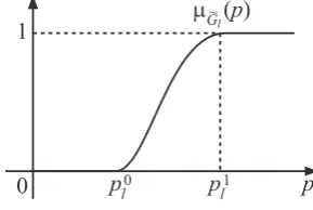
µG˜l(p) =
0 if p≤p0l gl(p) if p0l ≤p≤p
1
l, l= 1, . . . , k
1 if p1
l ≤p,
[image:3.595.88.260.234.290.2](8) where gl(p), l = 1, . . . , k are nondecreasing functions.
Fig. 2 illustrates a possible shape of the membership function for the fuzzy goal ˜Gl.
0
1
p
l1p
l0p
µ
(
Gp
)
l
~
Figure 2. An example of a membership function µG˜l(p) of a fuzzy goal ˜Gl
Recalling that the membership function is regarded as a possibility distribution, the degree of possibility that the probability ˜Pl attains the fuzzy goal ˜Glis expressed
as ΠP˜
l( ˜Gl), supp l
min{µP˜
l(pl), µG˜l(pl)} l= 1, . . . , k.
(9) Fig. 3 illustrates the degree of possibility ΠP˜
l( ˜Gl).
[image:3.595.94.264.371.492.2] [image:3.595.356.501.537.634.2]0
1
p
l1p
l0p
µ
(
Gp
)
l
~
µ
(
Pp
)
l
~
Π
P(
G
)
l
[image:4.595.43.288.251.446.2]~
~
Figure 3. The degree of possibility ΠP˜l( ˜Gl)
probability, we consider the possibility-based probabil-ity model for multiobjective random fuzzy integer pro-gramming problems formulated as
maximize ΠP˜1( ˜G1) · · · · maximize ΠP˜k( ˜Gk)
subject to Ax≤b, x≥0
(10)
or equivalently maximize h1
.. . maximize hk
subject to ΠP˜l( ˜Gl)≥hl, l= 1, . . . , k
Ax≤b, x≥0
(11)
5
Interactive
fuzzy
satisficing
method
Observing that (11) can be regarded as a multiobjec-tive programming problem, a complete optimal solution that simultaneously minimizes all of the objective func-tions does not always exist when the objective funcfunc-tions conflict with each other. Thus, instead of a complete optimal solution, a solution concept of Pareto optimal-ity plays an important role in multiobjective program-ming [5].
To be more specific, in the general form of multiob-jective programming problem
minimize z1(x) · · · · minimize zk(x)
subject to x∈X
(12)
where X denotes the set of all feasible solutions, since there does not always exist a solution minimizing all of the objective functions simultaneously, the solution concept of Pareto optimality plays an important role and it is defined as follows.
Definition 2 (Pareto optimal solution) A point
x∗ ∈ X is said to be a Pareto optimal solution if and only if there does not exist another x ∈ X such that
zi(x)≤zi(x∗)for alli∈ {1, . . . , k} andzj(x)̸=zj(x∗)
for at least onej∈ {1, . . . , k}.
As can be seen from Definition 2, in general there ex-ist an infinite number of Pareto optimal solutions if the feasible region X is not empty. In real-world decision
making problems, to make a reasonable decision or im-plement a desirable scheme, the decision maker should select one point from among the set of Pareto optimal solutions [5].
For the multiobjective programming problem (11) under consideration, in order to generate a candidate for the satisficing solution which is also Pareto opti-mal, the DM is asked to specify the reference levels of
hl, l = 1, . . . , k, called reference possibility levels. For
the reference levels ˆhl, l= 1, . . . , kspecified by the DM,
the corresponding Pareto optimal solution, which is, in the minimax sense, nearest ito the requirement or bet-ter than that if the reference possibility levels are at-tainable, is obtained by solving the augmented minimax problem [5]
minimize max
l=1,...,k
{
ˆ
hl−hl+ρ k
∑
l=1
(ˆhl−hl)
}
subject to ΠP˜
l( ˜Gl)≥hl, l= 1, . . . , k
Ax≤b, x≥0
(13) whereρis a sufficiently small positive number.
It should be noted here that (13) involves the pos-sibility constraints ΠP˜
l( ˜Gl) ≥ hl, l = 1, . . . , k,
solu-tion methods for ordinary mathematical programming problems cannot be directly applied. Realizing such dif-ficulty, we deal with the possibility constraints in the following way.
From (9), the possibility constraints ΠP˜l( ˜Gl) ≥ hl
in (11) or (13) are equivalently replaced by the condi-tions that there exists a pl such thatµP˜l(pl)≥ hl and
µG˜
l(p)≥hl, namely,
sup
sl
min
1≤j≤n
{
µMlj˜ (slj) |pl=P(ω|ul(ω)≤fl),
¯
ul∼N
(∑n
j=1
sljxj, n
∑
j=1
σ2ljx2j
)
≥hl (14)
and pl ≥µ⋆G˜l(hl), where sl= (sl1, . . . , sln) and µ⋆G˜l(hl)
is a pseudo inverse function defined as µ⋆
˜
Gl(hl) =
sup{pl | µG˜l(pl) ≥ hl}. This implies that there exists
a vector (pl,sl,u¯l) such that
min
1≤j≤nµM˜lj(slj)≥hl,u¯l∼N ∑n
j=1
sljxj, n
∑
j=1
σlj2x2j
,
pl=P(ω |ul(ω)≤fl), pl≥µ⋆G˜
l(hl),
which can be equivalently transformed into the condition that there exists a vector (sl,u¯l) such that
µM˜
lj(slj)≥hl, j= 1, . . . , n,
¯
ul∼N
∑n
j=1
sljxj, n
∑
j=1
σlj2x2j
,
P(ω |ul(ω)≤fl)≥µ⋆G˜l(hl). (15)
In view of (3), it follows that
where L (hl) and R (hl) are pseudo inverse functions
defined as L⋆(h
l) = sup{t | L(t) ≥ hl} and R⋆(hl) =
sup{t|R(t)≥hl}. Hence, (15) is rewritten as the
equiv-alent condition that there exists a ¯ul such that
P(ω| ul(ω)≤fl)≥µ⋆G˜l(hl),
¯
ul∼N
∑n
j=1
{mlj−L⋆(hl)αlj}xj, n
∑
j=1
σ2ljx2j
. (16)
SinceP(ω |ul(ω)≤fl) is transformed into
P ω
ul(ω)− n
∑
j=1
{mlj−L⋆(hl)αlj}xj
v u u t∑n
j=1 σ2 ljx 2 j ≤
fl− n
∑
j=1
{mlj−L⋆(hl)αlj}xj
v u u t∑n
j=1
σ2
ljx2j
,
in consideration of ¯
ul− n
∑
j=1
{mlj−L⋆(hl)αlj}xj
v u u t∑n
j=1
σ2
ljx
2
j
∼N(0,1),
(16) is equivalently transformed as
Φ
fl− n
∑
j=1
{mlj−L⋆(hl)αlj}xj
v u u t∑n
j=1 σ2 ljx 2 j
≥µ⋆G˜
l(hl), (17)
where Φ is a probability distribution function of the standard Gaussian random variableN(0,1).
From the monotone increasingness of Φ, (17) is rewrit-ten as
n
∑
j=1
{mlj−L⋆(hl)αlj}xj+ Φ−1(µ⋆G˜
l(hl)) v u u t∑n
j=1
σlj2x2j ≤fl,
(18) where Φ−1 is the inverse function of Φ.
In this way, the augmented minimax problem (13) is equivalently transformed into
minimize max
l=1,...,k
{
ˆ
hl−hl+ρ k
∑
l=1
(ˆhl−hl)
}
subject to
n
∑
j=1
{mlj−L⋆(hl)αlj}xj
+Φ−1(µ⋆
˜
Gl
(hl))
v u u t∑n
j=1
σlj2x2j ≤fl,
l= 1, . . . , k Ax≤b, x≥0
(19)
Observing that (19) is an ordinary nonconvex non-linear programming problem, it is possible to employ particle swarm optimization for nonlinear programming (PSONLP) [22] for obtaining an approximate solution.
Following the above discussions, we can now construct an interactive algorithm for deriving the satisficing solu-tion for the DM from among the Pareto optimal solusolu-tion set.
Interactive fuzzy satisficing method
Step 1: Ask the DM to specify the target valuesfl,l=
1, . . . , k, and determine the membership functions
µG˜l,l= 1, . . . , k.
Step 2: Set the initial reference possibility levels at 1s, which can be viewed as the ideal values, i.e., ˆhl =
1, l= 1, . . . , k.
Step 3: For the current reference possibility levels ˆhl,
l = 1, . . . , k, solve the corresponding augmented minimax problem (19).
Step 4: The DM is supplied with the corresponding Pareto optimal solution x∗. If the DM is sat-isfied with the current objective function values
h∗l, l = 1, . . . , k, then stop. Otherwise, ask the DM to update the reference possibility levels ˆhl,
l= 1, . . . , kby considering the current values of ob-jective functionshl, l= 1, . . . , k, and return to step
3.
It should be noted for the DM that any improvement of one objective function value can be achieved only at the expense of at least one of the other objective function values for the fixed target valuesfl, l= 1, . . . , k.
6
Numerical Example
In order to demonstrate the feasibility and efficiency of the proposed interactive fuzzy satisficing method, as a numerical example of (2), consider the two-objective random fuzzy linear programming problem formulated as:
minimize C¯˜1x minimize C¯˜2x subject to a1x ≤ b1
a2x ≤ b2 a3x ≤ b3 a4x ≤ b4
x= (x1, x2, x3, x4, x5, x6)T ≥0.
(20)
Table 1 shows values of coefficients of constraints ai,
i = 1,2,3,4 and bi, i = 1,2,3,4 and Table 2 shows
values of parameters of random fuzzy variablesmlj,αlj
and σ2
lj, l = 1,2, j = 1,2,3,4,5,6, where triangular
Table 1. Values of coefficients in constraints
ai1 ai2 ai3 ai4 ai5 ai6 b
a1 1.00 3.00 4.00 2.00 5.00 2.00 120
a2 2.00 4.00 5.00 1.00 9.00 8.00 250
a3 5.00 2.00 1.00 4.00 5.00 8.00 400
[image:6.595.41.291.174.265.2]a4 3.00 8.00 4.00 7.00 8.00 6.00 600
Table 2. Values ofmlj,αlj andσ2lj.
¯ ˜
cl1 ¯˜cl2 ¯˜cl3 c˜¯l4 ¯˜cl5 ¯˜cl6
m1j −7.30 −4.50 −5.00 −3.30 −5.50 −3.8
m2j 2.50 4.20 3.00 4.90 2.50 4.30
α1j 0.70 0.50 0.80 0.40 0.70 0.60
α2j 0.90 0.80 0.70 0.40 0.60 0.50
σ21j 1.40 1.00 1.10 1.20 1.10 0.90
σ22j 1.00 1.00 1.20 1.20 0.80 1.00
Through the use of this numerical example, it is now appropriate to illustrate the proposed interactive fuzzy satisficing method.
The parameter values of particle swarm optimization for nonlinear programming (PSONLP) are set as swarm sizeN = 50, maximal search generation numberTmax= 3000,c1= 2.0,c2= 2.0,w0= 1.2 andwTmax = 0.1.
Suppose that the DM sets the target values fl, l =
1,2 as f1 =−300, f2 = 100, and determines the linear membership functionsµG˜l,l= 1,2.
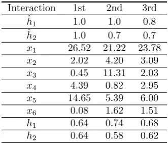
For the initial reference possibility levels ˆhl= 1, l=
1,2, the corresponding augmented minimax problem is solved, and the obtained result is shown at the column labeled “1st” in Table 3. DM is not satisfied with these values of objective functions, and the DM updates the reference probability levels as (1.0, 0.7) for improving the values of objective functionsh1at the expense ofh2. For the updated reference fractile levels, the corresponding augmented minimax problem is solved, and the obtained result is shown at the column labeled “2nd” in Table 3. A similar procedure continues until the DM is satisfied with the values of objective functions. In this example, we assume that the satisficing solution for the DM is derived in the third interaction.
Table 3. Interaction process.
Interaction 1st 2nd 3rd ˆ
h1 1.0 1.0 0.8 ˆ
h2 1.0 0.7 0.7
x1 26.52 21.22 23.78
x2 2.02 4.20 3.09
x3 0.45 11.31 2.03
x4 4.39 0.82 2.95
x5 14.65 5.39 6.00
x6 0.08 1.62 1.51
h1 0.64 0.74 0.68
h2 0.64 0.58 0.62
7
Conclusions
In this paper, random fuzzy multiobjective linear pro-gramming problems have been considered. For tack-ling the formulated problems, it has been assumed that the decision maker concerns about the probabilities that each of the objective function values is smaller than or equal to a certain target value. By introducing the fuzzy goals of the decision maker for the probabilities and as-suming that the decision maker is willing to maximize the degrees of possibility with respect to the attained probability, an interactive fuzzy satisficing method has been presented for deriving a satisficing solution for the decision maker by updating the reference possibility lev-els. It was shown that all of the problems to be solved in the proposed interactive fuzzy satisficing method can be solved through particle swarm optimization for nonlin-ear programming (PSONLP). An illustrative numerical example was provided to demonstrate the feasibility of the proposed method. However, further computational experiences should be carried out for several types of nu-merical examples. From such experiences the proposed computational method must be revised. Applications of the proposed method to the real world decision making situations will be required in the near future. Exten-sions to other stochastic programming models will be considered elsewhere. Also extensions to integer pro-gramming problems involving random fuzzy variable co-efficients will be required in the near future.
REFERENCES
[1] J.R. Birge, F. Louveaux, Introduction to Stochastic Programming, Springer, London, 1997.
[2] P. Kall, J. Mayer, Stochastic Linear Programming:
Models, Theory, and Computation, 2nd Edition,
Springer, New York, 2011.
[3] I. M. Stancu-Minasian, Stochastic Programming with Multiple Objective Functions, D. Reidel Publishing Company, Dordrecht, 1984.
[4] I. M. Stancu-Minasian, Overview of different
ap-proaches for solving stochastic programming prob-lems with multiple objective functions, In R. Slowin-ski, J. Teghem, (Eds.), Stochastic Versus Fuzzy Ap-proaches to Multiobjective Mathematical Programming under Uncertainty, Kulwer Academic Publishers, Dor-drecht/Boston/London, 71–101, 1990.
[5] M. Sakawa, Fuzzy Sets and Interactive Multiobjective Optimization, Plenum Press, New York, 1993.
[6] H.-J. Zimmermann, Fuzzy programming and linear pro-gramming with several objective functions, Fuzzy Sets and Systems, Vol. 1, No. 1, pp. 45–55, 1978.
[7] H.-J. Zimmermann, Fuzzy Sets, Decision-Making and Expert Systems, Kluwer Academic Publishers, Boston, 1987.
[8] G.B. Dantzig, Linear programming under uncertainty, Management Science, Vol. 1, No. 3–4, pp.197–206, 1955.
[image:6.595.41.207.669.810.2][10] M. Sakawa, H. Yano, Interactive fuzzy satisficing method using augmented minimax problems and its ap-plication to environmental systems, IEEE Transactions on Systems, Man and Cybernetics, Vol. SMC-15, No. 6, pp. 720–729, 1985.
[11] M. Sakawa, K. Kato, Interactive fuzzy multi-objective stochastic linear programming, In C. Kahraman (Ed.), Fuzzy Multi-Criteria Decision Making - Theory and Ap-plications with Recent Developments -, Springer, New York, 375–408, 2008.
[12] M. Sakawa, K. Kato, I. Nishizaki, An interactive fuzzy satisficing method for multiobjective stochastic linear programming problems through an expectation model, European Journal of Operational Research, Vol. 145, No. 3, pp. 665–672, 2003.
[13] M. Sakawa, K. Kato, An interactive fuzzy satisficing method for multiobjective stochastic linear program-ming problems using chance constrained conditions, Journal of Multi-Criteria Decision Analysis, Vol.11, No. 3, pp. 125–137, 2002.
[14] M. Sakawa, K. Kato, H. Katagiri, An interactive fuzzy satisficing method for multiobjective linear pro-gramming problems with random variable coefficients through a probability maximization model, Fuzzy Sets and Systems, Vol. 146, No. 2, pp. 205–220, 2004.
[15] H. Kwakernaak, Fuzzy random variables - I. definitions and theorems, Information Sciences, Vol. 15, No. 1, pp. 1–29, 1978.
[16] M. L. Puri, D. A. Ralescu, Fuzzy random variables, Journal of Mathematical Analysis and Applications, Vol. 114, No. 2, pp. 409–422, 1986.
[17] G.-Y. Wang, Z. Qiao, Fuzzy programming with fuzzy random variable coefficients, Fuzzy Sets and Systems, Vol. 57, No. 3, pp. 295–311, 1993.
[18] Z. Qiao, Y. Zhang, G.-Y. Wang, On fuzzy random linear programming, Fuzzy Sets and Systems, Vol. 65, No. 1, pp. 31–49, 1994.
[19] B. Liu, Random fuzzy dependent-chance programming and its hybrid intelligent algorithm, Information Sci-ences, Vol. 141, No. 3–4, pp. 259–271, 2002.
[20] M. Sakawa, I. Nishizaki, H. Katagiri, Fuzzy Stochas-tic Multiobjective Programming, Springer, New York, 2011.
[21] S. Nahmias, Fuzzy variables, Fuzzy Sets and Systems, Vol. 1, No. 2, pp. 97–110, 1978.