Numerical solution of Solving Higher order Boundary
Value Problems using Collocation Methods
*Taiwo O. A., **Raji M. T and ***Adeniran, P. O
*Department of Mathematics, University of Ilorin
**Department of Mathematics and Statistics, The Oke Ogun Poly., Saki ***Department of Science Lab. Technology, The Oke Ogun Poly., Saki
Corresponding Author: [email protected]
DOI: 10.29322/IJSRP.8.3.2018.p7552
http://dx.doi.org/10.29322/IJSRP.8.3.2018.p7552
Abstract: This paper deals with the numerical solutions of solving higher order Boundary Value Problems by Standard
Collocation and Perturbed Collocation Methods. We mention the two collocation points as equally- spaced points with boundary points inclusive and equally-spaced points with boundary points non-inclusive. Also, we observed that the accuracy obtained by Perturbed Collocation Method was reasonable when compared with the exact solution. Numerical examples were given to illustrate the performance of the work.
Keyword: Boundary Value Problem (BVP), Collocation Method, Standard and Perturbed Collocation
Methods, Ordinary Differential Equation (ODE)
1. INTRODUCTION
Numerical analysis is a branch of mathematics that deals with providing approximations and solutions to problems in Mathematics, especially those for which analytic solutions do not exists (i.e are not readily obtained)
Some methods that are currently used in Numerical Analysis include- the Interpolation Methods, Iteration Methods, Finite Difference Methods e.t.c. We used the Standard and Perturbed Collocation Methods in solving Differential Equations in higher order Boundary Value Problems, as it will be seen latter in this work.
Mathematical problems arise in numerous practical situations, particularly in Science and Engineering, for many of these problems, the most appropriate method of solution may not be purely mathematical. There are so many different methods widely used that is numerical methods for calculating such problems. While these methods were based on mathematical reasoning; Also, they largely consist of straight forward computations, which can be followed without need of great mathematical insight. Therefore, numerical approach is very good for solving many problems and that is why we focus on both the Standard Collocation and Perturbed Collocation Methods, which are both numerical methods used in solving differential equations.
The relevant application of Boundary value Problem can be find in real life situation ranging from Science to Engineering fields where problems they model include: spring problems, electrical circuit problem, buoyancy problems to mention a few. To these problems, arriving at a close-form solution are not always feasible for the mere fact that quite a good number of these real life problems do not have analytical solution and even in the availability of these solutions, it is well known that these are not amenable to direct numerical interpretation and hence limited in their usefulness in practical applications ([15],[19]). Also, there are some of these differential equations for which the solution in terms of formula are so complicated that one often prefers to apply numerical methods ([5],[9],[18]). Owing to these facts, there is always the need to develop new numerical methods of solution and to improve on the existing ones.
The collocation methods has found extensive application in recent years presented in a series of papers, for example, in [2-9] for the case of numerical solution of Ordinary Differential Equations (ODEs) and in [4,9,10] for the case of numerical solution of Partial Differential Equations (PDEs).
section 5, there is error estimate, in section 6, we have illustrative examples are given and table of result were presented while conclusion drawn is in section 7.
2. COLLOCATION METHODS
The order of an Ordinary Differential Equation (ODE) is the highest derivative in the equation, and a Boundary Value Problem (BVP) is one that is specified at certain boundary points, with conditions attached to the boundary point.
Consider the fourth order Boundary value problem (BVP) of the form:
b
x
a
y
y
y
y
x
f
y
iv=
(
,
,
′
,
′′
,
′′′
),
≤
≤
1together with the boundary conditions
0
)
(
a
=
y
20
)
(
a
=
y
i 31
)
(
b
=
y
41
)
(
=
′
b
y
5where a and b are the boundary points, and 0 and 1 are the boundary conditions for the points a and b.
Collocation method as one of the broad class methods of Weighted Residual (MWR) evoloved as a variable techniques for the solution of a broad class of problem. The technique as adapted in this paper involves constructing approximating solution of the form:
∑
==
N ii i
N
x
a
x
y
0
)
(
6where N is the degree of the approximant and
i
=
0
(
1
)
N
.which forms a solution to the given equation (1), now equation 6 can be expanded depending on the value of N used to have,
N N N
x
a
a
x
a
x
a
x
y
=
+
+
2+
+
2 1 0
)
(
7which is then differentiated to the order of the original equation(1), and substituted into equation(1). Two methods of selecting these points are considered in the following sub-sections.
a. Collocating at equally-spaced point(Boundary points non-inclusive)
The technique here demands that instead of collocating at points on zeros of x, the collocation points are determined by the use of:
1
,
3
,
2
,
1
;
)
(
−
=
−
+
=
k
N
N
k
a
b
a
x
k
8Where a and b are respectively the lower and upper bound of the interval, N is the chosen degree of the solution.
It is to be noted that equation(8) yields points that are located within the interval of consideration without the inclusion of boundary points a and b.
b. Collocating at equally-spaced point (Boundary Points inclusive)
2
,
3
,
2
,
1
;
2
)
(
=
−
−
−
+
=
k
N
N
k
a
b
a
x
k
9Where all parameters are as defined above
3. STANDARD COLLOCATION METHODS
In this method we shall assume an approximate solution of the form in equation (6), where N is the degree of the approximant and
ai(i ≥ 0) are to be determined.
Thus, equation (6) is then substituted into equations (1)-(5) to have
))
(
),
(
),
(
),
(
,
(
)
(
/ // ///x
y
x
y
x
y
x
y
x
f
x
y
iv N N N NN
=
10together with the boundary conditions
α
=
)
(a
y
N 11/ /
)
(
a
=
α
y
N 12β
=
)
(b
y
N 13/ /
)
(
b
=
β
y
N 14Hence, equation (10) is then collocated at point
x
=
x
k, to have))
(
),
(
),
(
),
(
,
(
)
(
k k N k N/ k N// k ///N k ivN
x
f
x
y
x
y
x
y
x
y
x
y
=
15Where
;
1
,
2
,
3
,
3
2
)
(
−
=
−
−
+
=
k
N
N
k
a
b
a
x
k
16Thus, equation (15) gives rise to (N-3) algebraic system of equations, with (N + i) unknown constants.
Four extra equations are obtained using equations (11)-(14). Altogether, we obtain (N + 1) algebraic linear equation with (N +1) unknown constants. These (N + 1) algebraic equation are then solved using Gaussian elimination to obtain the unknown constant
ai(i ≥ 0) which are then substituted back into our approximate solution given by equation(6)
4. PERTURBED COLLOCATION METHODS
In this method we shall assume an approximate solution of the form in equation (6), where N is the degree of the approximant and
ai(i ≥ 0) are to be determined.
Thus, equation (6) is then substituted into equations (1)-(5) to have
)
(
))
(
),
(
),
(
),
(
,
(
)
(
x
f
x
y
x
y
/x
y
//x
y
///x
H
x
y
ivN=
N N N N+
N 17Where
H
N(x
)
is defined by)
(
)
(
)
(
)
(
)
(
x
1T
x
2T
1x
3T
2x
4T
3x
H
N=
τ
N+
τ
N−+
τ
N−+
τ
N−1
1
);
(
)
(
x
=
Cos
NCos
−1x
−
≤
x
≤
T
N 18Thus, equation(17) is then collocated at points
x
=
x
k, to have)
(
))
(
),
(
),
(
),
(
,
(
)
(
k k N k N/ k N// k ///N k N kiv
N
x
f
x
y
x
y
x
y
x
y
x
H
x
y
=
+
19Where
;
1
,
2
,
3
,
1
2
)
(
=
+
+
−
+
=
k
N
N
k
a
b
a
x
k
20Thus, equation (20) give rise to (N+1) algebraic system of equations, with (N + 5) unknown constants.
Four extra equations are obtained using equations (11)-(14). Altogether, we obtain (N +5) algebraic linear equation with (N +5) unknown constants. These (N + 5) algebraic equation are then solved using Gaussian elimination to obtain the unknown constant
ai(i ≥ 0) which are then substituted back into our approximate solution given by equation(6).
5. ERROR ESTIMATE
In this section, an error estimator for the approximate solution of (6) is obtained. We defined
e
N(
x
)
=
y
(
x
)
−
y
N(
x
)
as theerror function of the approximate solution
y
N(
x
)
toy
(x
)
, where,y
(x
)
is the exact solution andy
N(x
)
is the approximatesolution computed for various values of N.
6. NUMERICAL EXAMPLES
Given below are numerical examples to illustrate the simplicity and the applicability of the discussed method.
Example 1: Consider the fourth order boundary value problem
2
1800
1
)
(
3600
)
(
3601
)
(
x
y
x
y
x
x
y
iv−
′′′
+
=
+
21with boundary conditions
1
)
0
(
=
y
221
)
1
(
=
′
y
23)
1
(
5
.
1
)
1
(
Sinh
y
=
+
24)
1
(
1
)
1
(
Cosh
y
′
=
+
25with the exact solution
y
(
x
)
=
1
+
0
.
5
x
2+
Sinh
(
x
)
.TABLE OF VALUES (RESULTS)
Table 1 of example 1
X Exact Standard
method of case N = 6
Perturbed method of case N = 6
Error of Standard Method Error of Perturbed Method
0 1.0 1.0 1.0 0 0
0.1 1.10516675 1.105158218 1.105171239 8.532E-4 4.489E-6
0.2 1.221336003 1.221309009 1.221341159 2.6994E-5 5.156E-6
0.3 1.34920293 1.349472069 1.349511098 4.8224E-5 9.195E-6
0.6 1.816653582 1.816542761 1.816523029 1.10821E-5 1.306E-4 0.7 2.003583702 2.003449265 2.003414421 1.34437E-4 1.6928E-4 0.8 2.208105982 2.207945751 2.207913576 1.60231E-4 1.9241E-4 0.9 2.431516726 2.431331719 2.431317603 1.8501E-4 1.9912E-4 1.0 2.675201194 2.675000001 2.675000001 2.01193E-4 2.01193E-4
The above table observed that the order of errors of Standard Collocation Method and Perturbed Collocation Methods are almost the same, but that of Perturbed Method having a slightly greater degree of accuracy. The order of the power of the error starts at -6 and ends at -4 in table 1 as we move higher in the interval 0-1.
EXAMPLE 2: Consider the fourth order BVP
2
0
,
0
)
(
)
(
x
+
y
′′′
x
=
≤
x
≤
π
y
iv 26together with the boundary conditions
0
)
1
(
=
y
27)
0
2
(
π
=
y
28
0
)
0
(
5
)
0
(
−
′
=
′′′
y
y
29and
25
.
0
)
(
50
)
(
2−
2=
−
′′′
πy
πy
30with the exact solution of the problem given by
))
(
2
.
1
)
(
1
(
)
100
444
(
)
(
x
x
1x
Cos
x
Sin
x
[image:5.595.31.499.466.776.2]y
=
−
−−
−
−
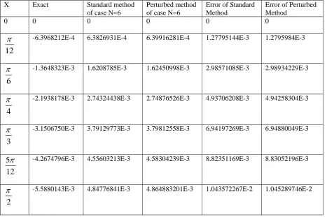
.Table 2 of Example 2
X Exact Standard method
of case N=6
Perturbed method of case N=6
Error of Standard Method
Error of Perturbed Method
0 0 0 0 0 0
12
π
-6.3968212E-4 6.3826931E-4 6.39916281E-4 1.27795144E-3 1.2795984E-36
π
-1.3648323E-3 1.6208785E-3 1.62450998E-3 2.98571085E-3 2.98934229E-34
π
-2.1938178E-3 2.74324438E-3 2.74876526E-3 4.93706208E-3 4.94258304E-33
π
-3.1506750E-3 3.79129773E-3 3.79812558E-3 6.94197269E-3 6.94880049E-312
5
π
-4.2674796E-3 4.55603213E-3 4.58304239E-3 8.82351169E-3 8.83052196E-32
The above table observed that the order of errors of Standard Collocation Method and Perturbed Collocation Method are almost the same, but that of Perturbed Method having a slightly greater degree of accuracy. The order of the power of the error starts at
power -3 and ends at -2 in table 2 as we move in the interval
2
0
−
π
.7. CONCLUSION
From table 1 and 2, it was observed that the Standard Collocation and Perturbed Collocation Method were both accurate methods (i.e Numerically) of solving higher order boundary value problems with the perturbed Collocation having slightly greater degree of accuracy than Standard Collocation Method, but Perturbed Collocation Method involving more tedious work when compared to the Standard Collocation Method.
REFERENCE
1. Atiknson K.E.(1978) “An Introduction to Numerical Analysis”. John Wiley and Sons N. Y.
2. Crisci M. R. (1992) “Stability Results for one step Discretized Collocation Methods in the
Numerical Treatment of Volterra Integral Equations”. Math. Comput. 58 (197) pp. 119-134. 3. Chuong N. M. and Tuan, N.V. (1995) “Spline Collocation Methods for Fredholm Integro-
Differential Equations of Second Order”, Acta Math. Vietnamica 20 (1) pp. 85-98. 4. Chuong N. M. and Tuan N. V (1997) “Spline Collocation Methods for Fredholm- Volterra integro-Differential Equations of High Order”, Vietnam J. Math. 25 (1) pp. 15-24.
5. David, S. B.(1987) “Finite Element Analysis from concepts to application”, AT & T Bell
Laboratory, Whippany, New Jersey.
6. Donald G and Vincenzo C.(1988) “Numerical Analysis for Applied Mathematics Science and
Engineering”. Addison Weley Publicity Company.
7. El-Daou M. K. and Khajah H. G (1997) “Iterated Solutions of Linear Operator Equations with the Tau Method”, Math. Comput. 66 (217) pp. 207-213.
8. Gottlieb D. and Orszag S. A (1986) “Numerical Analysis of Spectral Methods”, SIAM, Philadephia, 4th print.
9. Grewal, B.S.(2005) “Numerical methods in Engineering & Science”. 7th ed. Kanna Publishers, Delhi.
10. Hosseini Aliabadi M. and Ortiz, E. L. (1987) “On the Numerical Behavior of different
formulations of Tau Method for the treatment of Differential Inclusions”, Proceedings of the Second International Symposium on Numerical Analysis, Prague.
11. Hosseini Aliabadi M. and Ortiz, E. L. (1998) “Numerical treatment of Moving and Free
Boundary Value Problems with the Tau Method”, Computing Mathematical Application 35 (8) pp. 53-61. 12. Hosseini Aliabadi M. and Ortiz, E. L. (1988) “Numerical Solution of Feedback Control Systems
Equations”. Appl. Mathematics Lett. 1 (1) pp. 3-6.
13. Hosseini Aliabadi M. and Ortiz, E. L. (1991) “A Tau Method based on Non-Uniform Space
Time Elements for the Numerical Simulation of Solitons”, Comput. Math. Appl. 22 (9) pp. 7-19. 14. Hosseini Aliabadi M.(2000)”The Buchstab’s function and the Operational Tau Method”,
Korean J. Comput. Appl. Math. 7 (3) pp. 673-683.
15. Richard B.(2003) “Differential Equations”, Schaums Outline Series, McGRAW-HILL.
16. Sastry S. S.(1986)”Engineering Mathematics Volume II”. Prentice-Hall of India Private
N. Y.
18. Taiwo, O. A., Olagunju, A. S.(2012) “Chebyshev Methods for the numerical solution of
fourth-order differential equations”. International Journal of Physical Science. Vol. 7(13) pp. 2032-2037
19. Taiwo, O. A., Olagunju, A. S., Olotu, O. T., Aro, O. T.(2011) “Chebyshev Coefficient
Comparison Methods for the Numerical Solution of Non-Linear BVPs”. Pioneer JAAM. 3(2), pp 101-110.
20. Taiwo, O. A., and Raji, M. T.(2013)”Construction of Canonical Polynomial Basis functions for