USING DYNAMIC SYMBOLIC EXECUTION
by Scott Kausler
A thesis
submitted in partial fulfillment of the requirements for the degree of Master of Science in Computer Science
Boise State University
DEFENSE COMMITTEE AND FINAL READING APPROVALS
of the thesis submitted by
Scott Kausler
Thesis Title: Evaluation of String Constraint Solvers Using Dynamic Symbolic Execution
Date of Final Oral Examination: 2 May 2014
The following individuals read and discussed the thesis submitted by student Scott Kausler, and they evaluated his presentation and response to questions during the final oral examination. They found that the student passed the final oral examination.
Elena Sherman, Ph.D. Chair, Supervisory Committee Tim Andersen, Ph.D. Member, Supervisory Committee Dianxiang Xu, Ph.D. Member, Supervisory Committee
The author would first and foremost like to express his thanks to the Computer Science faculty at Boise State University. Specifically, the author would like to thank Dr. Elena Sherman for all of her effort in mentoring and assisting him on his research throughout the past year. The author also appreciates the support of his other committee members, Dr. Tim Anderson and Dr. Dianxiang Xu. In addition, he would like to thank Dr. Amit Jain for his aid throughout the admission process and the author’s first year of graduate school.
Obviously, comparisons of string constraint solvers would be impossible without any string constraint solvers. Therefore, the author thanks the developers of the string constraint solvers used for making their solvers available and for providing additional insight into their solvers. In particular, the author recognizes Muath Alkhalaf and his fellow STRANGER developers for providing insight into the differences of string constraint solvers. Finally, the author thanks his parents for their everlasting support and his brother for encouraging him to study computer science. This research was supported with funding from the IGEM grant.
Symbolic execution is a path sensitive program analysis technique used for error detection and test case generation. Symbolic execution tools rely on constraint solvers to determine the feasibility of program paths and generate concrete inputs for feasible paths. Therefore, the effectiveness of such tools depends on their constraint solvers.
Most modern constraint solvers for primitive data types, such as integers, are both efficient and accurate. However, the research on constraint solvers for complex data types, such as strings, is ongoing and less converged. For example, there are several types of string constraint solvers provided by researchers. However, a potential user of a string constraint solver likely has no comprehensive means to identify which solver would work best for a particular problem.
In order to help the user with selecting a solver, in addition to the commonly used performance criterion, we introduce two criteria: modeling cost and accuracy. Using these selection criteria, we evaluate four string constraint solvers in the context of symbolic execution. Our results show that, depending on the needs of the user, one solver might be more appropriate than another, yet no solver exhibits the best overall results. Hence, we suggest that the preferred approach to solving constraints for complex types is to execute all solvers in parallel and enable communication between solvers.
ABSTRACT . . . v
LIST OF TABLES . . . x
LIST OF FIGURES . . . xi
LIST OF ABBREVIATIONS . . . xiii
1 Introduction . . . 1
1.1 Symbolic Execution . . . 1
1.1.1 Description . . . 1
1.1.2 Example . . . 1
1.2 Constraint Solvers . . . 5
1.2.1 Constraint Solvers in Symbolic Execution . . . 5
1.3 String Constraint Solvers . . . 8
1.3.1 Example . . . 9
1.3.2 String Constraint Solver Characteristics . . . 11
1.3.3 String Constraint Solver Evaluation . . . 13
1.4 Dynamic Symbolic Execution . . . 14
1.5 Thesis Statement . . . 15
2 Current Tools and Methods . . . 17
2.1 Overview . . . 17
2.2.1 Examples . . . 22
2.2.2 Automata Solver Clients . . . 24
2.3 Bit-vector Based Solvers . . . 27
2.3.1 Examples . . . 27
2.3.2 Bit-vector Solver Clients . . . 29
2.4 Other Solvers . . . 30
2.4.1 Examples . . . 31
2.5 Related Work on Comparison of String Constraint Solvers . . . 31
3 Metrics for String Sovler Comparisons . . . 33
3.1 Example . . . 34
3.2 Performance . . . 37
3.3 Modeling Cost . . . 38
3.4 Accuracy . . . 39
3.5 Measurements of Accuracy . . . 41
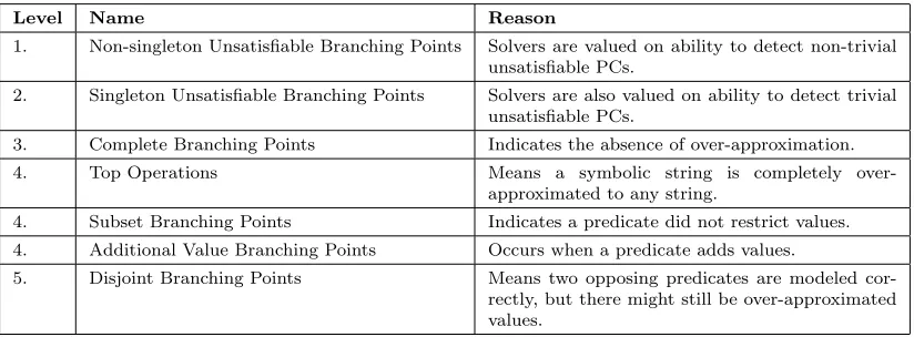
3.5.1 Measure 1: Unsatisfiable Branching Points . . . 41
3.5.2 Measure 2: Singleton Branching Points . . . 42
3.5.3 Measure 3: Disjoint Branching Points . . . 44
3.5.4 Measure 4: Complete Branching Points . . . 44
3.5.5 Measure 5: Subset Branching Points . . . 45
3.5.6 Measure 6: Additional Value Branching Points . . . 47
3.5.7 Measure 7: Top Operations . . . 48
3.5.8 Hierarchy of Accuracy . . . 49
3.6 Dynamically Comparing Solvers . . . 50
4.1 Overview . . . 53
4.2 Instrumenter . . . 55
4.3 Collector . . . 59
4.4 Processor . . . 60
4.5 Constraint Solvers . . . 61
4.5.1 EJSA . . . 68
4.5.2 ESTRANGER . . . 73
4.5.3 EZ3-str . . . 76
4.5.4 EECLiPSe-str . . . 78
4.6 Summary . . . 79
5 The Evaluator . . . 80
5.1 Performance . . . 80
5.2 Modeling Cost . . . 81
5.3 Measurements of Accuracy . . . 82
5.3.1 Measure 1: Unsatisfiable Branching Points . . . 82
5.3.2 Measure 2: Singleton Branching Points . . . 83
5.3.3 Measure 3: Disjoint Branching Points . . . 83
5.3.4 Measure 4: Complete Branching Points . . . 84
5.3.5 Measure 5: Subset Branching Points . . . 85
5.3.6 Measure 6: Additional Value Branching Points . . . 85
5.3.7 Measure 7: Top Operations . . . 85
5.4 Debugging . . . 86
5.5 Summary . . . 88
6.1 Modeling Cost . . . 90
6.2 Performance . . . 94
6.3 Accuracy . . . 96
6.4 Recommendations . . . 100
7 Conclusion and Future Work . . . 105
7.1 Comparison of String Constraint Solvers . . . 105
7.2 Future Work . . . 106
7.2.1 Comparisons . . . 106
7.2.2 Constraint Solver Development . . . 107
7.3 Final Note . . . 108
REFERENCES . . . 109
3.1 Variations in modeling cost, accuracy, and performance. . . 34 3.2 Displays the importance of each measurement of accuracy. . . 49
4.1 Available interfaces used in the extended solvers. . . 66 4.2 Describes the methods modeled by each extended string constraint solver.67
6.1 Program artifacts and constraint descriptions. . . 90
1.1 An integer based code snippet that may be explore using SE. . . 2
1.2 A symbolic execution tree for the code in Figure 1.1. . . 3
1.3 Demonstrates a SQL query generated using JDBC that could produce a runtime error due to a missing space between address and WHERE. . 9
2.1 Example code snippet. . . 18
2.2 Constraint graph for the code snippet in Figure 2.1. . . 18
2.3 Automaton representing any string. . . 21
2.4 Nodeterministic automaton representing “foo”. . . 21
2.5 Nondeterministic automaton representing “foo” concatenated with any string. . . 21
3.1 A disjoint branching point. . . 40
3.2 A non-disjoint branching point. . . 40
3.3 Approximation affects satisfiability result. . . 40
3.4 Approximation does not affect satisfiability result. . . 40
3.5 A code snippet that demonstrates a singleton branching point and a singleton hotspot. . . 43
3.6 A subset branching point that falls under case one. . . 46
3.7 A subset branching point that falls under case two. . . 46
4.1 Diagram of SSAF. . . 52
4.3 Demonstrates three-address code. . . 56 4.4 Instrumented code and the corresponding CG. Based on code in Figure 2.1.58 4.5 Nodeterministic automata that were independently created by
extract-ing the first two and last character of the strextract-ing “foo”. . . 64 4.6 Nodeterministic automaton representing “foo” after “bar” has been
inserted at index 2. . . 64 4.7 Nondeterministic automaton representing “foo” after ignore case
op-eration. . . 72
5.1 An unsound branching point. . . 87
6.1 Uses methods encountered on the x-axis to display modeling cost and characteristics of our test suite. . . 91 6.2 Y-axis displays the average time per branching point in seconds. . . 94 6.3 Y-axis displays the median time per branching point in seconds. . . 95 6.4 A code snippet that will not produce unsatisfiable branching points. . . . 101 6.5 Displays accuracy in our test suite. . . 104
API– Application Programming Interface
BDD – Binary Decision Diagram
BEA – Beasties
CG – Constraint Graph
CLP – Constraint Logic Programming
CSP– Constraint Satisfaction Problem
DFA – Deterministic Finite Automata
DSE – Dynamic Symbolic Execution
FG – Flow Graph
HCL – HtmlCleaner
ITE – iText
JHP – Jericho HTML Parser
JNA – Java Native Access
JPF – Java PathFinder
JSA – Java String Analyzer
JST – Java String Testing
JXM – jxml2sql
M2L – Monadic Second-Order Logic
MPJ – MathParser Java
MQG – MathQuiz Game
NCL – Natural CLI
NFA – Nondeterministic Finite Automata
OCL – Object Constraint Language
parray – Paramertized Array
PC – Path Condition
SE – Symbolic Execution
SML – String Manipulation Library
SMT – Satisfiability Modulo Theory
SPC– Symbolic PathFinder
SSAF – String Solver Analysis Framework
CHAPTER 1
INTRODUCTION
1.1
Symbolic Execution
1.1.1 Description
Symbolic execution (SE) [26, 10] is a path sensitive static program analysis technique that is useful for error detection, test case generation, and SQL injection attack generation. SE interprets programs using symbolic instead of concrete input values, e.g., numbers. These symbolic values are initially unrestricted, i.e., they can represent any concrete value. Upon reaching a branching point, i.e., a conditional statement, SE follows either a true or false branch. When following the selected branch, SE generates a constraint corresponding to that branch and conjoins it with the constraints of the previously taken branches. Thus, the resulting conjunction of constraints, called the path condition or PC, is the conjunction of all constraints along the explored path. A PC represents all concrete values that variables can evaluate to at that point during concrete executions that follow the same path.
1.1.2 Example
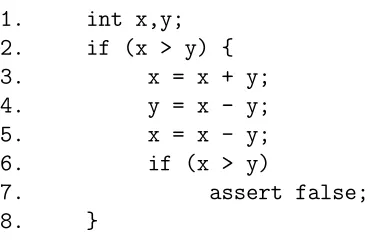
1. int x,y;
2. if (x > y) {
3. x = x + y;
4. y = x - y;
5. x = x - y;
6. if (x > y)
7. assert false;
8. }
Figure 1.1: An integer based code snippet that may be explore using SE.
consider how the code in Figure 1.1 is analyzed by SE. Figure 1.2 depicts the code’s SE tree [30]. At line 1, SE assigns symbolic values X for variable x and Y for variable y. In concrete execution, i.e., when executing a program normally, X and Y are concrete values, but in SE we cannot make any assumptions about these values because we want to reason about all potential concrete values for x and y. The symbolic values are initially unrestricted and the PC is initially assigned to true. However, at line 2, two separate constraints are generated and independently extend the PC to reflect the outcome of each branch. The first branch, represented by node 3 in Figure 1.2, assumes the branching point at line 2 is true, so the PC is conjoined with the constraintX > Y. The second branch, which leads to node 8a in Figure 1.2, assumes the branching point is false and conjoins the PC with the constraintX ≤Y. We now have two separate PCs that represent two different paths.
1) [P C :true]x=X, y =Y
2) [P C :true]X > Y?
8a) [P C :X ≤Y]EN D 3) [P C :X > Y]x=X+Y, y =Y true
false
4) [P C :X > Y]y=X+Y −Y =X, x=X+Y
5) [P C :X > Y]x=X+Y −X =Y, y =X
6) [P C :X > Y]Y > X?
8b) [P C :X > Y ∧Y ≤X]EN D 7) [P C :X > Y ∧Y > X]EN D true
false
Figure 1.2: A symbolic execution tree for the code in Figure 1.1.
Notice that the symbolic values for x and y are now swapped due to the assignment statements in lines 3-5 so that x has symbolic valueY and y has symbolic value X.
These updated symbolic values forxandyare used in the generation of constraints for the branching point at line 6. At line 6, the constraintY ≤X is added to the PC to generate the false condition. The final PC for the true branch of the first branching point and the false branch of the second branching point now statesX > Y ∧Y ≤X. In some cases, SE might refine this PC to a simpler form, i.e.,X > Y.
that path.
In order to detect infeasible paths such as the true branch at line 6 in Figure 1.1, SE must use a constraint solver to solve the conjunction of constraints. If the constraint solver can detect an unsatisfiable PC, it reports this result to the SE tool. Furthermore, SE uses a constraint solver to find values that might occur at a hotspot, which we define as follows:
Definition 1.1. Ahotspot is a program point where an interesting value or expression is located.
An error or injection attack can be found by conjoining the PC at a hotspot with an error or injection attack pattern, and a test case can be found by generating inputs that lead to a hotspot.
The ability to detect unsatisfiable PCs is an essential feature in SE. If a constraint solver is used to detect an error by solving a constraint, and it incorrectly reports that the constraint is satisfiable, then we say it has produced a false positive, which essentially means the constraint solver’s result caused the SE tool to report an error that doesn’t exist. For example, if we use SE to detect an error at a hotspot by conjoining constraints that represent an error pattern to a PC, then SE will always report that an error is present if its constraint solver cannot detect an unsatisfiable PC, regardless of if there is an actual error.
explosion problem, only programs with few branching points can be fully analyzed by SE. In particular, identifying all paths that traverse a loop is difficult because each iteration of a loop may generate a new path.
To make SE more efficient, bounds on the number of loop iterations to be explored are used. This limits the number of paths to be explored. The example based on Figure 1.1 shows another technique employed by SE to limit the number of paths to be explored and improve efficiency: using a constraint solver to detect and ignore infeasible paths. Neither technique affects SE’s time complexity. Because SE uses constraint solvers to improve efficiency and solve PCs at hotspots, the effectiveness of a SE tool is dependent on its constraint solvers.
1.2
Constraint Solvers
1.2.1 Constraint Solvers in Symbolic Execution
When SE makes use of a constraint solver to solve constraints, it enters its second phase, called the constraint solving phase. There are two cases that cause SE to enter the constraint solving phase. The first case is when the SE tool performs a check to determine if a PC is satisfiable when a branching point is encountered. The second case is when the SE tool encounters a hotspot. At a hotspot, the constraint solver is often used to generate test cases, generate injection attacks, or detect errors.
and produces a solution, i.e., concrete values of symbolic values, that satisfies the PC. In addition, some constraint solvers may report a solution for all concrete values that are represented by a symbolic value in a PC, instead of just one.
In order to generate test cases, a constraint solver returns concrete values for initial symbolic values in a satisfiable PC, e.g., 1 for X in the example given for Figure 1.1. These concrete values can then be used to execute the program along the same path represented by the PC.
In order to detect an error or injection attack at a hotspot, invalid patterns can be encoded as a set of constraints then conjoined with a PC. Any satisfying assignment for this conjoined constraint represents a value that is both invalid and satisfies the original PC, i.e., it indicates the presence of an error or injection attack. Constraint solvers that are capable of producing values that lead to a hotspot, i.e., concrete assignments to initial symbolic values, can also produce an invalid set of inputs.
We now present several definitions that will be used throughout the remainder of this thesis:
Definition 1.2. A sound constraint solver will never report that a satisfiable PC is unsatisfiable.
Definition 1.3. A complete constraint solver will never report that an unsatisfiable PC is satisfiable. A complete constraint solver will never report any false positives, i.e., it does not produce any solutions that cannot evaluate a PC to true.
Definition 1.4. An accurate constraint solver is both sound and complete.
Definition 1.6. Under-approximation occurs when a solution of a constraint is complete but unsound. An under-approximated solution might miss concrete values that occur given a PC but does not add extra concrete values.
As a rule, constraint solvers must be sound but may or may not be complete, meaning a constraint solver must report all values that actually occur given the constraint but may include extra values, i.e., values may be over-approximated but never under-approximated. This means that a trivial (but useless) constraint solver can report that all paths are satisfiable and any value can occur at any hotspot. If a solver is unsound, it will report that a satisfiable PC is unsatisfiable, might not produce any test cases, and might report that there are no invalid patterns at a hotspot, when in reality there is one or more.
In general, determining if a given PC is satisfiable is an undecidable problem. For example, a constraint in the theory of linear integer arithmetic is decidable, but adding a multiplication symbol to its signature makes it non-linear integer arithmetic, which is undecidable [38]. Because determining the satisfiability of a PC is an undecidable problem, we may approximate PCs and allow results that are not complete.
1.3
String Constraint Solvers
In this thesis, we apply string constraint solvers to string constraints gathered from Java programs. This means that we analyzed variables and methods that come from
the java.lang.String,java.lang.StringBuilder, and java.lang.StringBuffer
classes. These classes describe our string types. For brevity, we may respectively refer to these classes as String, StringBuilder, or StringBuffer. When referring to methods in these classes, we use the name and parameter type to denote a specific method, i.e., substring(int). In addition, we use only the name when referring to all methods that share that name, e.g., substring refers to substring(int) and
substring(int,int). We do not refer to the calling classes or return values of these
methods because we do not need to distinguish methods using classes or return values. There are several methods present in multiple string classes, e.g., append appears in
both StringBuilder and StringBuffer, but in these cases the same approach is
taken regardless of the class.
String theory is not well defined because every programming language contains a unique library of predicates, such as contains(String), and operations, such as
trim(), that may be applied to strings. Although any program that uses strings
false positives. An example of the importance of complete string constraint solvers is demonstrated below.
1.3.1 Example
1. public void printAddresses(int id) throws SQLException {
2. Connection con = DriverManager.getConnection("students.db");
3. String q = "SELECT * FROM address";
4. if(id!=0)
5. q = q + "WHERE studentid=" + id;
6. ResultSet rs = con.createStatement().executeQuery(q);
7. while(rs.next()){
8. System.out.println(rs.getString("addr"));
9. }
10. }
Figure 1.3: Demonstrates a SQL query generated using JDBC that could produce a runtime error due to a missing space betweenaddress and WHERE.
Consider the code presented in Figure 1.3, which was initially featured as an example in [9]. This code uses JDBC to print addresses stored in a database of students. Line 2 creates the database connection to “students.db”, line 3 starts an SQL query using the String class, line 5 appends the query with a WHERE clause if the conditional statement at line 4 evaluates to true, line 6 executes the query, and lines 7-9 print the “addr” column of the query’s result. The Java syntax is valid and will not cause a compilation error.
Appending the WHERE clause to the query results in a error. Queries containing the WHERE clause read as:
“SELECT * FROM addressWHERE studentid=” + id, where id != 0
Notice that there is no space between “address” and “WHERE”. Without this space, the query is not valid SQL syntax and causes a runtime exception when the statement is executed at line 6.
Now, imagine this code gets interpreted by a SE tool. Assume a hotspot is created whenever the executeQuery method is called. If there is a case where
printAddressesis called with id != 0, the symbolic value generated at the hotspot in
line 6 will contain the value “SELECT * FROM addressWHERE studentid=” + id. Given standard regular language operations where∼represents negation,·represents concatenation,εrepresents the empty string,∗represents Kleene closure,∪represents disjunction, [a−b] represents any numeral betweena and b (inclusive), and concrete strings are surrounded by “”, assume the regular expression constraint∼(“SELECT * FROM address” · (ε ∪ “ WHERE studentid=” · (ε ∪ “-”) · [1−9]· [0−9]∗)) is conjoined with the PC for the hotspot at line 6. Because the regular expression matches strings that are NOT of the form “SELECT * FROM address” or “SELECT * FROM address WHERE studentid=” + id, the resulting symbolic value will still contain “SELECT * FROM addressWHERE studentid=” + id. The SE tool should report that the error pattern is satisfiable, which will alert the user that a potential error has occurred. Ideally, the user will run a concrete execution of the program with values that will cause this error and verify that it exists.
several potential error values that do not cause errors. For example, it may report an error when id = 0. If the tester tests this case instead of the case where id != 0, he or she may falsely conclude that there is no error at that point.
1.3.2 String Constraint Solver Characteristics
SE tools work on different abstraction levels when modeling string constraints. Some precisely model string constraints by representing a string as an array of characters and exploring string library functions as a set of primitive functions. This approach can be inefficient, so other tools use string constraint solvers that work in a particular fragment of the theory of strings.
For example, a basic string constraint solver may only support concatenation
and containment[18], while a more advanced string constraint solver might support
concatenation, containment, replace, substring, and length [47, 50]. These
more advanced string constraint solvers can model many predicates and operations in theString,StringBuilder, and StringBuffer classes, although the accuracy of the model depends on the accuracy of the basic predicates or operations. For example,
anendsWith predicate can usually be modeled accurately usingconcatenation and
containment. String constraint solvers also commonly support constraints in the
form of regular expressions [9, 24], which are useful for describing error patterns, describing injection attack patterns, or modeling predicates and operations.
an operation is modeled as a modification to an automaton. Automata-based string constraint solvers are efficient because the time complexity of modifying an automaton is usually polynomial in the number of states and/or transitions in the automaton.
On the other hand, bit-vector string constraint solvers work by imposing a length bound on the characters in a symbolic value, encoding predicates and operations in some underlying formalism, such as satisfiability modulo theory (SMT) or constraint satisfaction problems (CSP), searching for a solution, and increasing the length bound if no solution is found until a maximum length k is reached. If at that point no solutions can be found, the result is unsatisfiable. This length requirement allows bit-vector string constraint solvers to naturally keep track of the length of the underlying string, whereas automata-based string constraint solvers must use other techniques to keep track of a string’s length.
Unfortunately, this length requirement also causes bit-vector solvers to be ineffi-cient. In order to support multiple variables, which is a requirement in a constraint solver for SE, bit-vector solvers must iterate over every combination of lengths. Usually, this iteration requires more time than SE will allow, so bit-vector solvers must take an alternate approach to be used in SE. Such alternate approaches often involve solving any constraints on length before encoding a string as a bounded bit-vector [6]. A constraint solver may or may not incrementally solve constraints in a PC. An incremental constraint solver can store a previous conjunction of constraints in an intermediate form. This intermediate form allows the user to add one constraint at a time to a PC while still collecting the result of the entire PC. This is advantageous for reusing the prefix of a PC. A PC prefix is defined as follows:
c1∧. . .∧ci, where 1≤i < k.
Incrementally solving constraints saves time when solving PCs that contain the same prefix. Because SE attempts to explore every path in the program, it often reuses prefixes, so it benefits from using an incremental constraint solver. An automaton may serve as an intermediate form, so automata-based string constraint solvers are naturally incremental.
1.3.3 String Constraint Solver Evaluation
Despite the underlying differences, all string constraint solvers may be evaluated using the same metrics. These metrics fall under the categories of performance, modeling cost, and accuracy.
Performance can be measured by keeping track of the time required for evaluation of several PCs. However, complications arise when comparing incremental and non-incremental constraint solvers. In order to compare performance of both types of solvers, for incremental solvers we incrementally keep track of the time required to evaluate the whole PC, instead of only measuring the time required to add a constraint to the PC. In order to make our analysis diverse, we measure PCs taken from long program paths.
Modeling cost is based on the effort required to use a constraint solver. This is a useful metric for comparison because users want to spend as little time as possible understanding and extending a constraint solver for use in their analyses.
are at least partially sound. However, in general, we assume the solvers are sound. Therefore, our measures of accuracy deal with observing over-approximation.
There are two causes of over-approximation. The first cause is from an incomplete model of an operation. It is hard to tell which operations are over-approximated by a string constraint solver, so we must assume over-approximation is introduced in all future constraints that involve a modified symbolic value.
The second cause of over-approximation comes from predicates at branching points. Fortunetely, we know that if complementary predicates for a branching point create two disjoint sets from the values represented by a symbolic value, then the branching point has not be over-approximated. Therefore, when the constraints generated by two branches of a branching point do not create disjoint sets of values, we must assume over-approximation has been generated from the predicate for at least one branch. In addition, we must assume this over-approximation is propagated to future constraints that use the symbolic values represented by the two branches.
Although SE can be used to compare string constraint solvers, it is not the most optimal technique when using real world programs for comparison because of its tendency to only use simple PCs representing short program paths. In addition, there is no means of gathering concrete values in SE, which help in determining if a solver is accurate. Instead, we prefer to use a technique that generates PCs based on concrete execution, called dynamic symbolic execution, which we introduce in the next section.
1.4
Dynamic Symbolic Execution
execution of the program. DSE treats all input values as symbolic, even though concrete execution consists of concrete inputs.
DSE collects constraints as the program follows its execution path, which requires instrumentation of the program [20]. Program instrumentation is a technique that inserts additional statements into a program to collect certain attributes. In this case, the attributes are the constraints encountered in the program’s execution.
Because DSE follows the program’s actual execution, there is no need to check if a branch is feasible during concrete execution with DSE, since a branch must be feasible to execute it in concrete execution. In addition, DSE allows us to compare symbolic values to the actual values of variables at a given program point. Moreover, because DSE only follows one concrete path, it can analyze nontrivial PCs generated by following long paths in a program’s execution. This makes it more scalable than SE. The combination of these advantages allow DSE to essentially be used to test values generated by a constraint solver, which leads us to the thesis statement.
1.5
Thesis Statement
For this thesis, the following three criteria, which we describe in Chapters 3 and 5, will be used to compare the extended string constraints solvers in Chapter 4, which are based on solvers presented in Chapter 2, and our results will be presented in Chapter 6:
• Performance: How does a solver’s average time for solving PCs compare to the
• Modeling Cost: Which solver requires the least effort to model string methods?
Why might one solver require more effort than another?
CHAPTER 2
CURRENT TOOLS AND METHODS
2.1
Overview
This chapter first describes works related to string constraint solvers, along with analyses that the solvers are used in. Next, it presents works in comparisons of string constraint solvers. The analyses detailed in this chapter often use a constraint graph (CG) to describe PCs, which we defined below:
Definition 2.1. A constraint graph is a directed graph where all source vertices represent either symbolic or concrete values and all remaining vertices represent either operations or predicates encountered during execution. An edge represents the flow of data from one vertex to another.
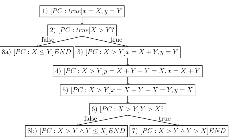
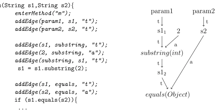
m(String s1,String s2){ s1 = s1.substring(2);
if (s1.equals(s2)) { ...
Figure 2.1: Example code snippet.
S1 2
substring(int) target
arg
S2
equals(Object) arg
target
Figure 2.2: Constraint graph for the code snippet in Figure 2.1.
between s1 and s2, and the symbolic state of each variable is updated to reflect the result.
Figure 2.2 presents a CG for the code in Figure 2.1. In this figure, the vertices labeled S1 and S2 represent initial symbolic values for variables s1 and s2. In addition, the 2 vertex represents a concrete integer value, since that value is the same in every program execution. The edges in this figure represent the flow of data from one vertex to another, i.e., they indicate that the value from one vertex is used in another vertex. The target and arg edge labels respectively denote the calling symbolic string and the argument for each method. Finally, thesubstring(int) and equals(Object) vertices represent string methods (substring(int) denotes an operation and equals(Object) denotes a predicate). Notice that the CG captures the value returned by the substring(int) operation with a target edge leading to the equals(Object) predicate, and S2 is the argument for equals(Object).
The CG in Figure 2.2 represents only one CG for a particular program execution. In fact, different analyses use different CGs, depending on the data they want to capture. In this way, a CG is only an abstraction of the program used to represent the data required to achieve the goals of the analysis.
computation that depends on data obtained from a taint source is tainted. Other values are considered to be untainted. A taint policy determines how taint flows through a program execution.
Just like the CG depends on the type of analysis, the result of a taint analysis depends on the taint policy. For example, most taint analyses will considers1 ands2 to be initially tainted in Figure 2.1, since they represent unknown input. Furthermore, some taint policies will consider s1 to be tainted after the substring(int) operation because it is dependent on s1’s initial value. On the other hand, some policies might consider values to be untainted after the operation because it could remove potentially harmful values that might occur for s1.
If we use a conservative taint policy, then all vertices in our CG from Figure 2.2, except for 2, get tainted. Because it does not depend on user input, 2 should not be tainted. Under this conservative policy, s1 propagates taint to the substring(int) and equals(Object) vertices while s2 propagates taint to theequals(Object) vertex.
String constraint solvers use various underlying representations of symbolic strings. We therefore present our survey of the solvers based on their underlying representations. These solvers are often used in SE, static analysis, dynamic analysis, and model driven analysis. Before reviewing the solvers, we must first introduce what the terms static analysis, dynamic analysis, and model driven analysis mean.
Because static analysis might over-approximate the values of variables, it is often used in web security analyses. For example, static analysis on strings is used to detect SQL injection attacks, since this type of attack is prevalent across the Web and often times does not depend on non-string types.
On the other hand, dynamic analysis is an analysis performed on an executing program. Dynamic analysis is often used to circumvent the limitations of static analysis. Namely, it is less resource intensive, capable of analyzing deep program paths, and allows comparisons of values taken from real world programs.
Instead of analyzing programs,model driven analysis analyzes models of programs. For example, it might be used to generate test cases using a program model created with a modeling language. Interest in model driven analysis was sparked by the popularity of other analysis techniques.
The remainder of this chapter is structured as follows. First, we introduce the string constraint solvers that use each representation of symbolic strings, i.e., we introduce each type of string constraint solver. After introducing a type of solver, we provide a survey of analyses that the type of solver is used in. Finally, we present related work on comparison of string constraint solvers.
2.2
Automata-Based Solvers
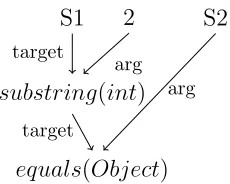
An automata-based string constraint solver uses automata to represent symbolic and concrete string values. For example, an unrestricted symbolic value can be represented with the automaton shown in Figure 2.3. A nondeterministic automaton representing the concrete string “foo” is shown in Figure 2.4.
Start .
Figure 2.3: Automaton representing any string.
Start ‘f’ ‘o’ ‘o’
Figure 2.4: Nodeterministic automaton representing “foo”.
Start ‘f’ ‘o’ ‘o’ ε
.
Figure 2.5: Nondeterministic automaton representing “foo” concatenated with any string.
are not defined for traditional automata theory. These operations manipulate the states and transitions in an automaton to model the set of strings that occur after a string method is used. For example, several automata-based string constraint solvers support substringoperations. All automata-based string constraint solvers support
concatenation, so we use the automata from Figures 2.3 and 2.4 to demonstrate this
2.2.1 Examples
Christensen et al. [9] use multi-level finite automata to represent strings. Using multi-level finite automata, a minimal deterministic automaton that describes all possible values of a string variable at that program location can be extracted for every hotspot. The resulting library of automata operations is referred to as Java String Analyzer (JSA). JSA’s automata are pointer based and use ranges of character values to represent transitions.
Haderach is a prototype created by Shannon et al. [37] that uses JSA as the underlying automata library, but with one major modification. In order to more accurately express its predicates and operations, it maintains dependencies among automata. This approach increases accuracy because changes that occur late in a PC can be applied to previous automata.
Redelinghuys et al. [33] also extend JSA in their analysis. Their extension accepts a set of constraints and returns a SAT/UNSAT result along with string values, since JSA was not designed to do this. They also enhance JSA with their own routines, but do not describe what enhancements were made.
unsatisfiable. Non-linear numeric constraints are handled by a randomized solver or a regular linear solver after being converted to a linear form.
Yu et al. [47, 48, 45, 46] present STRANGER, which uses its string manipulation library (SML) to handle string and automata operations, such as replacement,
concatenation, prefix, suffix, intersection, union, and widen1. The SML,
which we refer to as STRANGER for brevity, uses the MONA library [3] to represent deterministic finite automata (DFA). In MONA, transitions are represented using Binary Decision Diagrams (BDDs).
In order to more precisely model predicates such as the not equals predicate, Yu et al. [49] introduce multi-track automata for solving string constraints. In a multi-track automaton, each track corresponds to one string value. Although this approach is empirically shown to be more precise than a standard automata approach, it is also more resource intensive.
Hooimeijer and Weimer [18] create an automata-based decision procedure for subset and concatenation constraints, as well as a prototype called DPRLE. This is the only constraint solver based on automata with proven correctness of its algorithms.
Tateishi et al. [40] create an analysis that uses a BDD-based automata represen-tation of Monadic Second-Order Logic (M2L) formulae. This implemenrepresen-tation uses MONA as the underlying library. The advantage of this approach is that it can create conservative, i.e., over-approximated, models of operations and is powerful enough to model methods such as Java’s replace methods.
1The SML is now open source and available at https://github.com/vlab-cs-ucsb/Stranger.
2.2.2 Automata Solver Clients
Symbolic Execution
Shannon et al. [37] integrate symbolic strings into a SE prototype named Haderach. Traditionally in SE, the PC is stored explicitly as a list of constraints. However, Haderach represents string constraints by manipulating finite-state automata. A symbolic value’s automaton therefore accepts all strings that satisfy the PC for the associated variable. Haderach extends the code base of Juzi [23], which is a prototype designed to repair structurally complex data that comes from complicated structures, such as red-black trees.
Static Analysis
Christensen et al. [9] present a static program analysis technique to demonstrate the applicability of approximating the values of Java string expressions. Their analysis builds a CG to capture the flow of strings and string operations. This CG consists of Init nodes to represent new string values,Join nodes to capture assignments (or other join points),Concatnodes to represent string concatenation, and bothUnaryOp
and BinaryOp nodes to represent other string operations. After building their CG,
the authors construct a context-free grammar, approximate it as a regular grammar, and extract automata from this regular grammar.
STRANGER [47, 48, 45, 46] is an automata-based string analysis tool that can prove an application is free from specified attacks or generate a pattern characterizing malicious inputs. STRANGER uses Pixy [22] to parse a PHP program and construct a dependency graph of string operations and values with a taint analyzer. Cyclic dependencies in the graph are replaced with strongly connected components. A vul-nerability analysis is conducted on the now acyclic dependency graph. In this graph, nodes are processed in a topological order using automata operations. These nodes could represent null, assign, concat, replace, restrict, and input operations. Both a forward and a backward analysis may be performed using STRANGER.
monitor checks dynamically generated queries against the model and rejects queries that violate the model. This is done by parsing the actual string into SQL string tokens then checking if the model’s automaton accepts it.
Tateishi et al. [40] perform a static analysis that is not based on a CG. Instead, the analysis encodes string assignments as operations in M2L. After the encoding, a solver is applied to check for satisfiability.
An automated static analysis technique for finding SQL injection attacks in PHP is presented by Wassermann and Su [43]. This analysis combines static taint analysis with string analysis. In order to identify substrings that may have been tainted by user input, a CG is used to maintain the relation between variables. This analyses uses Minamide [28] to model string operations.
Dynamic Analysis
Kiezun et al. [25] create a tool called Ardilla. Ardilla dynamically creates inputs that expose SQL injection and cross site scripting attacks for PHP. It executes the program with arbitrary inputs, generates constraints based on the path followed, negates a previously observed constraint, and solves the new set of constraints to mutate inputs. A taint propagator is then used to detect potential user inputs. Taint may be removed using sanitizers. Finally, candidate attack patterns are generated and verified.
and adjusts future inputs to cover those branches by taking the first unexecuted path on the next execution. Strings, records, and database relations are immutable and manipulated using an abstract data type that allows creation, comparison, and
concatenation of strings. All statements are classified as either a halt, input,
assignment, conditional, database manipulation, or abort statement. The
constraints gathered from DSE are used to create satisfying assignments and update both the input map and database. This ensures the program gets tested while the database is in several different states.
2.3
Bit-vector Based Solvers
Bit-vector solvers encode string constraints in terms of some underlying logic, e.g., SMT, but the translation requires a bounded length on strings. This length bound allows string operations that would otherwise be undecidable but is a limitation for these solvers since they ignore solutions outside of their length bound. However, useful analyses can still be performed with these solvers, particularly if the length bound is large. Furthermore, this restriction on string length has motivated the development of solvers that do not suffer from this limitation, as we discuss in Section 2.4.
The solvers detailed below vary based on the logic and underlying representation of symbolic strings. However, each of the solvers below encodes each string as a vector.
2.3.1 Examples
primi-tivesShiftandFuse. First, the axioms for the constraints are tested for satisfiability. If they are satisfiable, Pex then extracts values, unfolds quantifiers, and attempts to find solutions up to a bounded length.
HAMPI [24] is a bit-vector solver capable of expressing constraints in regular languages and fixed size context free languages. It works by normalizing constraints into a core form, encoding them into bit-vector logic, and using the STP [13] solver to solve the bit-vector constraints. HAMPI originally only supportedconcatenation on single symbolic variables along with its regular and context free constraints, but the current version also supports substring operations and multiple fixed length symbolic variables. HAMPI works in an NP-complete logic for its core string constraints.
Redelinghuys et al. [33] build a bit-vector based string constraint solver that uses Z3. Their implementation uses Z3’s array support to solve for multiple string lengths simultaneously.
Kaluza [34] works in three steps. First, it translates string concatenation constraints into a layout of variables. Second, it extracts integer constraints on the lengths of strings to find a satisfying length assignment. Finally, Kaluza translates the string constraints into bit-vector constraints to check for satisfiability. The bit-vector constraints are solved by repeatedly invoking HAMPI.
Ulher and Dave [41] reimplement HAMPI as SHAMPI. This is done in order to demonstrate the utility of the Smten tool, which automatically translates high-level symbolic computation into SMT queries.
support length, concatenation, indexed substring,containment, andequality operations. There are three cases where the solver solves constraints. In the first case, every valid length assignment yields a solution. In the second case, the solver can detect an unsatisfiability based purely on length constraints. In the final case, the solver generally performs poorly because elements have to be incrementally assigned values before being checked for satisfiability. Since the aforementioned solver is unnamed, we refer to it as ECLiPSe-str from this point on.
Li and Ghosh [27] use a new structure, called a paramertized array (parray), to represent a symbolic string in their solver, called PASS. Parrays map symbolic indices to symbolic characters and use symbolic lengths. Constraints are encoded as quantified expressions. In addition, quantifier elimination is used to convert universally quantified constraints into a form that can easily be processed by SMT solvers. The algorithm used to solve these expressions is guaranteed to terminate because its search space is bounded by length. The advantage of this approach is that it can be used to detect unsatisfiable constraints quickly. Use of automata was avoided because they tend to over-approximate values, have weak length connections, do not extract relations between values, and must enumerate values. However, automata are still required to encode regular expressions. Automata are also used to determine unsatisfiability quickly, i.e., in cases where parrays perform poorly. These automata can be converted into parrrays as needed.
2.3.2 Bit-vector Solver Clients
Symbolic Execution
the event space of user interactions using a GUI explorer. After that, the dynamic symbolic interpreter records a concrete execution of the program with concrete inputs. Kudzu tracks each branching point, modifies one of the branching points, and uses a constraint solver to find inputs that lead to the new path, so that it can cover a program’s input value space. It then intersects symbolic values with attack patterns at hotspots in order to detect potential vulnerabilities.
Model Driven Analysis
In order to ensure model correctness in generating test cases based on model-driven engineering, Gonzalez et al. present EMFtoCSP2 in [15]. EMPtoCSP is based on
CLP. User inputs include the model, the set of constraints over the model, and the properties to be checked. EMF3 and Object Constraint Language (OCL)4
parsers are used to translate this input. After translation, the code is sent to the ECLiPSe5 constraint programming framework to check if the model holds with the given properties. A visual display of a valid instance is then given. This display can be used as input to a program to be tested.
2.4
Other Solvers
As previously mentioned, this class of solver was developed to circumvent the limita-tions of bit-vector solvers. Because the length is not bounded, a more general theory must be used to impose string constraints.
2http://code.google.com/a/eclipselabs.org/p/emftocsp 3http://www.eclipse.org/modeling/emf
2.4.1 Examples
Z3-str [50] treats strings as a primitive type within Z3. It uses Z3’s theory of uninterpreted functions and equivalence classes to determine satisfiability. Z3-str systematically breaks down constants and variables to denote sub-structures until the breakdown bounds the variables with constant strings or characters. When concat is detected by the Z3 core, the abstract syntax tree is passed to Z3-str using a call back function. Z3-str then applies the concat rule, reduces the tree, and sends it back to Z3’s core. The split function adds a rule as the disjunction of all possible split strings. To solve, Z3-str either finds a concrete string in an equivalence class or simplifies formulas and assigns values to free variables. Substring is represented by breaking the argument into three pieces, asserting the middle piece is the return string, and asserting the proper lengths for the other pieces. Contains checks if one string is a substring of another. When contains is negated, solutions are generated for the free variables and post processing is used to check if one symbolic string is contained within the other.
2.5
Related Work on Comparison of String Constraint
Solvers
Hooimeijer and Veanes [17] also evaluate the performance of different automata-based constraint solvers on basic automata operations. The authors conclude that a BDD-based representation works well when paired with lazy intersection and difference algorithms. Chapter 6 of this thesis gives another picture of performance comparisons between automata encodings.
Redelinghuys et al. [33] compare the performance of their custom implementations of bit-vector constraint solvers and their custom extension of JSA in the context of SPF. The result is that different types of solvers perform better in separate situations, and the authors conclude that the choice of decision procedure is not important.
Zheng et al. [50] compare Z3-str with Kaluza. The comparison is done both in terms of performance and correctness, although the authors do not define the latter. Z3-str outperforms Kaluza in 13 out of 14 test cases.
Choi et al. [8] make a comparison of their approach with JSA based on performance and precision. In this case, the authors use the generality of regular expressions to determine which solver is more precise. In all cases, their approach is at least as precise as JSA. In addition, their approach is more efficient than JSA in all but one test case.
CHAPTER 3
METRICS FOR STRING SOVLER COMPARISONS
As we previously discussed, the majority the comparisons between constraint solvers are based on performance. This metric is important from the perspective of constraint solver developers, since solver competitions [39] mainly focus on performance. Even though performance is important for users, other metrics can also play critical roles in an effective constraint solver. We speculate that at least two additional metrics, modeling cost and accuracy, should be considered when selecting an adequate solver. In this chapter, we explain in detail what they are and why they are important.
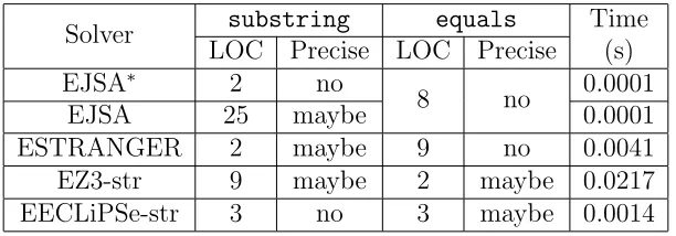
Solver substring equals Time LOC Precise LOC Precise (s)
EJSA∗ 2 no
8 no 0.0001
EJSA 25 maybe 0.0001
ESTRANGER 2 maybe 9 no 0.0041
EZ3-str 9 maybe 2 maybe 0.0217 EECLiPSe-str 3 no 3 maybe 0.0014
Table 3.1: Variations in modeling cost, accuracy, and performance.
3.1
Example
In order to demonstrate the importance of all three metrics in string solver com-parisons, we illustrate the type of string constraints that SE can generate using the code snippet in Figure 2.1. Recall that in SE the input values for variables s1 and s2 of method m(String s1, String s2) are symbolic values S1 and S2. After the substring operation, s1’s symbolic value gets updated to reflect the substring operation. To explore the true branch of the conditional statement, SE generates the following constraint:
(S1.substring(2)).equals(S2) (3.1)
This constraint restricts the concrete values of s1 to those whose substrings starting at index 2 are the same as the concrete values of s2. To determine whether it is possible to assign valuesS1 and S2 that can satisfy such relation betweens1 and s2, i.e., whether the true branch is feasible, SE passes the above constraint to a string constraint solver.
two displays the modeling cost in terms of number of lines of code (LOC) used to extend thesubstring(int)method for each extension, while column three describes accuracy by telling whether the extension might be precise or not. Columns four and five provide a similar description for the equals(Object) method. The last column shows performance as the average time in seconds that the extended string solvers require to process the two methods after ten queries. We represent accuracy in terms of the precision of method implementation, which we label as “maybe” or “no”. For
equals(Object), we consider the precision of models in both the predicate and its
negation. If we are certain that the model is imprecise then we label it with “no”. Otherwise, we label it with “maybe” because we lack the formal proofs required to conclusively state that the models are precise.
In this example, we have two versions of JSA extensions for the substring(int) method. The first, EJSA∗, uses the built-in method, which only requires a couple of LOC to invoke. JSA’s native modeling of this method over-approximates the result by allowing the resulting automaton to represent any length postfix of the original automaton, not just a single substring. For example, if the symbolic string S1 from the example based on Figure 2.1 was constrained to represent the concrete string “foo”, the symbolic string after the native modeling of substring(2) would represent concrete strings “foo”, “oo”, “o”, and “”.
of correctness for this algorithm, we mark it as “maybe” accurate. Note that implementing a more precise model of thesubstringmethods required a substantial amount of effort. This effort includes the labor of writing code in addition to other efforts, such as understanding the theory of automata.
Unlike JSA, STRANGER already provides a model of substringwith no obvious approximations. Therefore, to achieve the same level of accuracy, we used significantly less effort to model this string operation. However, neither of our automata-based solvers could model the equals method without introducing over-approximation. This is because automata-based solvers cannot easily capture the complex interaction between symbolic values in the false conditions of predicates such as this one and are forced to over-approximate to remain sound. We provide an explanation of this over-approximation in Section 4.5.1.
For EZ3-str, we found no obvious over-approximation for either of the two methods. Z3-str comes with a direct interface for the substring operation, equals predicate, and negation operator. Therefore, the substring operation in Figure 2.1 can be modeled using Z3-str’s built in interface along with Z3’s symbolic integer type. Furthermore, the equals predicate is modeled using Z3-str’s equals interface, and the predicate’s negation is modeled by applying the negation operator to the original predicate.
In EECLiPSe-str, we could not model the substring(int) method without introducing clear over-approximation. ECLiPSe-str cannot model it precisely because its substring method must return a string of at least length one. Since the empty string is a feasible result, a sound model must over-approximate the method by disjoining the result with the empty string.
string solver extensions. EZ3-str has the worst performance when processessing the constraint but also models the string methods with the best precision. EJSA definitely displays the best performance while maintaining the same precision as ESTRANGER. EECLiPSe-str comes in second in the performance category with a level of accuracy that is incomparable to that of the automata-based solvers.
This example illustrates the tight coupling between modeling cost and accuracy, i.e., higher modeling cost results in higher precision, which in its turn should make a solver more accurate. It also shows the coupling between accuracy and performance, i.e., the most accurate solver took the longest time to execute. Also, the example shows that solvers with the same level of accuracy don’t necessarily exhibit the same performance, i.e., EJSA and ESTRANGER have similar accuracy but ESTRANGER performs worse. Moreover, there are situations when the solvers’ accuracies are not comparable. Hence, the performance, i.e., the average times, cannot be judged fairly in such circumstances. We use this example to illustrate the differences in several solvers and by no means make conclusions about these four solvers. In the following sections, we describe in detail what metrics we use to perform comparisons of the four extended string constraint solvers.
3.2
Performance
paths, since PCs for such paths include several complex constraints. For example, a program path containing hundreds of branching points might cause SE to run out of resources. Therefore, the performance of constraint solvers is relatively unknown for these long paths. Analysis of performance on long program paths is useful because SE is constantly improving and, therefore, is constantly exploring longer paths. Thus, we aim to make our performance comparison unique by analyzing PCs gathered from long program paths.
3.3
Modeling Cost
We define a modeling of a constraint as follows:
Definition 3.1. Modeling is expressing a predicate or operation in terms of a constraint solver’s interface.
Essentially, modeling is the translation from the language of the problem to the language of the solver. Since the solvers were developed to solve specific problems, we expect that the effort required by a user to model a different problem, i.e., modeling cost, should vary by solver.
string method, the method may not be supported adequately in the context of the problem. For example, Z3-str supports areplaceoperation, but its support is limited and non-applicable in the context of SE of Java programs.
Obviously, the more effort the user invests in extending a solver, the more precise the solver can model the user’s problem. Thus, our extra effort in reimplementing
the substring operation in EJSA results in a more precise model of the operation
compared to JSA’s native one, which in turn allows EJSA to produce more accurate results. Lack of effort might result in poor modeling.
3.4
Accuracy
The accuracy of a solver’s results depends on the precision of its models. When a solver can precisely model all string methods, it is both sound and complete, i.e., it never reports that a satisfiable constraint is unsatisfiable and that an unsatisfiable constraint is satisfiable. In other words, if there is a solution, then the solver will find it. If a solver is sound but incomplete, we say that it over-approximates, i.e., it might return SAT when it should return UNSAT, and if a solver is complete but unsound, then we say it under-approximates, i.e., it might return UNSAT when it should return SAT.
Naturally, poorly modeled methods negatively affect the accuracy of the solver. Conceptually, imprecise modeling of string operations and predicates reduces the solver’s accuracy. For instance, when a solver cannot precisely model a predicate such
as equals, the solution set for a constraint with this imprecisely modeled predicate
original (S)
S2 S1
Figure 3.1: A disjoint branching point.
original (S)
S2 S1
Figure 3.2: A non-disjoint branch-ing point.
new mapping (S) original
S2 S1
Figure 3.3: Approximation affects satisfiability result.
new mapping (S) original
S2 S1
Figure 3.4: Approximation does not affect satisfiability result.
gray semicircle depicts over-approximated values not present in a precisely modeled predicate shown in Figure 3.1. In the case where a solver cannot precisely model an operation, the symbolic string after the operation will contain additional string values that might affect reasoning about a branching point, as depicted in Figure 3.3, or might not, as shown in Figure 3.4.
characters are likely restricted due to STRANGER’s underlying structure.
Since neither the developers of the four solvers provide formal proofs that their implementations are correct nor we prove the correctness of our extensions, we attempt to evaluate the accuracy of the solvers empirically. The ideal way to experimentally evaluate the accuracy of a solver is to compare its set of solutions for a constraint to the accurate set of solutions. However, since the solution oracle cannot be obtained, we propose nine conservative measurements that can be use to conjecture about solvers’ accuracy in the context of SE. These measurements are presented in the next section.
3.5
Measurements of Accuracy
We describe these measurements of accuracy so that future users of constraint solvers can adapt their choice measurements when using the solver, i.e., as a means of accuracy evaluation. Furthermore, these measurements may be used in future work on comparison of constraint solvers.
In the following subsections, we refer to two constraint solvers Σ1 and Σ2 for use in
comparisons of accuracy. We then formally define conditions under which one solver is more accurate than another using the “/” symbol.
3.5.1 Measure 1: Unsatisfiable Branching Points
such as SE, but if a constraint solver reports a PC is UNSAT, we can trust the result to be accurate as long as we trust that the constraint solver is sound.
Since we assume our solvers are sound, our first measure of accuracy is the number of unsatisfiable PCs that a solver can detect. If one solver Σ2 evaluates a constraint
as SAT and another Σ1 as UNSAT, then we say that the latter is more accurate than
the former, i.e., Σ2 /unsat Σ1. The ability of a solver to detect unsatisfiable PCs is
crucial for SE, since it prevents SE from exploring infeasible paths. We refer to the branching points where a solver can detect that one of the outcomes is unsatisfiable as unsatisfiable.
We see in Figures 3.1 to 3.4 that before a branching point a symbolic value represents a set of valuesS. In a constraint solver, the models of opposing predicates will create symbolic values that represent two new sets S1 and S2. An unsatisfiable branching point indicates that S1≡ ∅ orS2≡ ∅.
3.5.2 Measure 2: Singleton Branching Points
Furthermore, in order to assess the complexity of the PCs in unsatisfiable branching points, we check whether all symbolic string values involved in a branching point contain only a single concrete string value. If this is not the case, then evaluation of the constraint is nontrivial and the unsatisfiable branching point is marked as non-singleton. Otherwise, we say the branching point is singleton. Therefore, if a solver Σ1 can detect an unsatisfiable PC at a non-singleton branching point, then
Σ1 has higher accuracy than a solver Σ2 that can detect an unsatisfiable PC at a
singleton branching point, i.e., Σ2/singleΣ1.
other words, a singleton branching point reflects the case seen in concrete execution, where only one path is satisfiable with the input values.
In addition, only non-null values can generally be passed into Java string methods. Therefore, we can assume that no over-approximation is present at a singleton branching point that uses one such method.
Hotspots may also be singleton as long as each symbolic value involved only maps to one concrete value. However, we do not introduce singleton hotspots as their own measurement of accuracy because they are calculated in the same way as a singleton branching point. With that said, there is one caveat: programmers often intentionally use concrete values at hotspots.
1. if (s1.equals("foo"))
2. if(!s1.equals("bar"))
3. System.out.println("hello");
Figure 3.5: A code snippet that demonstrates a singleton branching point and a singleton hotspot.
3.5.3 Measure 3: Disjoint Branching Points
The third measure of accuracy evaluates whether or not a solver can partition the domains of symbolic strings at a branching point and directly checks if the second cause of over-approximation described in Section 1.3.3 has produced inaccurate results at a branching point. If the set in the domain of one outcome of a branching point does not contain values from the set in the domain of the other outcome of the same branching point and vice versa, i.e., if the sets are disjoint, then we say that the solver was able to partition the domain, and it did not over-approximate at that point. We call such branching pointsdisjoint. Conceptually, a disjoint branching point is shown in Figure 3.1, while a non-disjoint branching point is presented in Figure 3.2.
For a more formal definition, suppose a symbolic value represents a set of strings S, and the two opposing predicates at a branching point separateS into two setsS1 and S2. The branching point is disjoint if S1∩S2≡ ∅.
We say that a solver Σ1 is more accurate than a solver Σ2 if the set of disjoint
branching points produced by Σ1 is a proper superset of Σ2’s disjoint branching point
set, i.e., Σ2 /disj Σ1. Note that an unsatisfiable branching point is a special case of a
disjoint branching point.
3.5.4 Measure 4: Complete Branching Points
over-approximated by an operation or predicate, then such over-approximation may cause a disjoint branching point to become non-disjoint and vise versa. Since we do not prove that models of string operations are precise, we conservatively assume that none of them are modeled precisely, and we have yet to find a method to empirically disprove this assumption.
Thus, we can only argue that the solver does not over-approximate when a disjoint branching point has never been preceded by either an operation or a non-disjoint branching point. We say this type of disjoint branching point is acomplete branching point. A complete branching point indicates that the result of a constraint solver is not over-approximated. For this accuracy measure, we say that a solver Σ1 is more
accurate than a solver Σ2 if the set of complete branching points for Σ1 is a proper
superset of the same set for Σ2, i.e., Σ2/compΣ1.
3.5.5 Measure 5: Subset Branching Points
Because different solvers use different decision procedures, some solvers may be capable of supporting extra measurements of accuracy. For example, an automaton is used to describe a set of strings, so automata-based string constraint solvers are naturally capable of using set operations. This subsection introduces a measure of accuracy that is based on set operations. Since only our automata-based solver extensions deal with sets, this measure of accuracy does not apply to EZ3-str and EECLiPSe-str.
original (S)
S2 S1
Figure 3.6: A subset branching point that falls under case one.
original (S)
S2 S1
Figure 3.7: A subset branching point that falls under case two.
set of values represented by S1 is a subset of the set of values represented by S2, or vice versa, i.e., S1 ⊂ S2 or S2 ⊂ S1. These branching points, which we refer to as subset branching points, indicate that the predicate modeled for at least one branch did not change the set of values represented by S, i.e. they indicate that S1≡S or S2 ≡ S. In other words, if the set in the domain of one outcome of the branching point is a subset of another outcome of the same branching point then we call the branching point a subset branching point.
Conceptually, a subset branching point is shown in Figures 3.6 and 3.7. In these figures, the original set is not constrained by one predicate. Instead, we assign all values in the set represented by the original symbolic value to the domain of the S2 branch, and over-approximated values in the figures are shown in gray. Because the set of values representing the S1 branch is a proper subset of the set of values from the original symbolic value, it is also a proper subset of the set of values representing the S2 branch.
Since the sets in the domains of both branches should contain different values, a subset branching point only occurs in a sound solver if the constraints describing one or more branches did not restrict the symbolic value occurring before the branching point. We say that solver Σ1 is more accurate than solver Σ2 if the set of subset
branching points for Σ2 is a proper superset of the set of subset branching points