Patron: Her Majesty The Queen Rothamsted Research Harpenden, Herts, AL5 2JQ
Telephone: +44 (0)1582 763133 Web: http://www.rothamsted.ac.uk/
Rothamsted Research is a Company Limited by Guarantee Registered Office: as above. Registered in England No. 2393175. Registered Charity No. 802038. VAT No. 197 4201 51. Founded in 1843 by John Bennet Lawes.
Rothamsted Repository Download
A - Papers appearing in refereed journals
Van Den Bosch, F., Mcroberts, N., Van Den Berg, F. and Madden, L. V.
2008. The basic reproduction number of plant pathogens: matrix
approaches to complex dynamics. Phytopathology. 98 (2), pp. 239-249.
The publisher's version can be accessed at:
•
https://dx.doi.org/10.1094/PHYTO-98-2-0239
The output can be accessed at:
https://repository.rothamsted.ac.uk/item/89xy5/the-
basic-reproduction-number-of-plant-pathogens-matrix-approaches-to-complex-dynamics
.
© Please contact [email protected] for copyright queries.
Analytical and Theoretical Plant Pathology
The Basic Reproduction Number of Plant Pathogens:
Matrix Approaches to Complex Dynamics
F. van den Bosch, N. McRoberts, F. van den Berg, and L. V. Madden
First and third authors: Department of Biomathematics and Bioinformatics, Rothamsted Research, Harpenden, AL5 2JQ, UK; second author: Scottish Agricultural College, King’s Buildings, West Mains Road, Edinburgh EH9 3JG, UK; and fourth author: Department of Plant Pathology, Ohio State University, Wooster, OH 44691-4096.
Accepted for publication 25 September 2007.
ABSTRACT
van den Bosch, F., McRoberts, N., van den Berg, F., and Madden, L. V. 2008. The basic reproduction number of plant pathogens: Matrix approaches to complex dynamics. Phytopathology 98:239-249.
The basic reproduction number, R0, is defined as the total number of infections arising from one newly infected individual introduced into a healthy (disease-free) host population. R0 is widely used in ecology and animal and human epidemiology, but has received far less attention in the plant pathology literature. Although the calculation of R0 in simple sys-tems is straightforward, the calculation in complex situations is challeng-ing. A very generic framework exists in the mathematical and
biomathe-matical literature, which is difficult to interpret and apply in specific cases. In this paper we describe a special case of this general framework involving the use of matrix population models. Leading by example, we explain the existing mathematical literature on this subject in such a way that plant pathologists can apply the method for a wide range of pathosystems.
Additional keywords: Beet necrotic yellow vein virus, comparative epi-demiology, cultivar mixture, landscape, nursery, propagator tree, Plum pox virus.
This paper describes a systematic method, originally developed by Diekmann et al. (8), to calculate the basic reproduction number from knowledge of the pathogen’s life-cycle and its interactions with the host plant (i.e., from knowledge of the disease cycle). The basic reproduction number, R0, is defined as
the total number of infections arising from one newly infected individual introduced into a healthy population. Rephrasing this definition, R0 is also the generation-to-generation multiplication
factor of the pathogen population at infinitesimally low pathogen density (i.e., at a density when propagules produced by the pathogen will not come in contact with host individuals previ-ously infected by the pathogen).
R0 is widely used in ecology and animal and human
epidemi-ology for several reasons. (i) The basic reproduction number defines the threshold, R0 = 1, between an epidemic (increase in
pathogen density), R0 > 1, and no epidemic, R0 < 1. When each
‘mother’ infection causes, on average, more than one ‘daughter’ infection, R0 exceeds 1, so the pathogen or disease population
density will increase. (ii) It is a useful parameter in comparative epidemiology, summarizing the life-cycle components and the interactions with the host into one metric signifying the patho-gen’s reproduction capacity. (iii) In many models (but not all), R0
can be used to determine the ultimate or steady-state value of disease or pathogen density in a host population (10,21,23, 26,27,34), and (iv) R0 is a simple tool to evaluate different disease
control methods within one coherent framework.
The concept behind the basic reproduction number goes back at least to Ross(33), who studied malaria epidemics. Vanderplank (36,37) introduced the metric into the plant pathology literature. In Vanderplank’s model, the corrected basic infection rate, Rc, is
the number of new infections caused per time-unit by one infec-tive infection, the parameter i is the length of the infectious period, which has the dimension of time. As discussed by Vanderplank, the product of these two, iRc, thus has the dimension
of numbers and is equal to the basic reproduction number, R0.
Vanderplank uses this quantity, which he terms the progeny-parent ratio as a basis for assessing disease control strategies. Although the work of Vanderplank dates back to the sixties and seventies, R0 is still not widely used by plant pathologists, in
general, despite the intuitive interpretation and application of the parameter. Several studies in botanical epidemiology have ad-dressed the use of R0 in recent years (13,14,15,22,26,28,30,34),
and the recent book by Madden et al. (27) discusses the calcu-lation of R0 for a range of epidemic models. The present paper
seeks to extend the range of techniques available to plant pathological research in this regard.
The calculation of R0 in cases with complex dynamics is not
straightforward. Examples of systems with complex dynamics include: (i) the presence of more than one host cultivar; (ii) large spatial scales (e.g., regions) with multiple fields; and (iii) propa-gator-tree-nursery systems. A procedure used to calculate R0 in
most cases in the plant pathology literature (13,14,15,28), is to: (i) develop a nonlinear model for pathogen dynamics (usually con-sisting of a system of nonlinear differential equations); (ii) calcu-late the steady-state where the pathogen is present (the internal steady-state); and (iii) from the steady-state expression derive a criterion (i.e., an inequality) showing the combination of model parameters in which the pathogen population density is larger than zero. This method, however, does not guarantee that the expression derived actually is R0. That the expression is the basic
reproduction number can only be ascertained by retrospectively finding a biological interpretation for the components of the
ex-Corresponding author: F. van den Bosch
E-mail address: [email protected]
* The e-Xtra logo stands for “electronic extra” and indicates that the online version contains programming scripts for finding the dominant or maximum eigenvalue of an n×n matrix and some other software tips for starting to use matrix projection models.
doi:10.1094 / PHYTO-98-2-0239
© 2008 The American Phytopathological Society
pression that convinces the researcher that it is R0. In Box 1, we
give a specific example clarifying the pitfalls of this approach. A very generic framework exists in the mathematical and biomathematical literature (8,16) for the calculation of R0 for
virtually any biologically relevant case. Though brilliant in its generality, this framework is abstract and difficult to interpret and apply in specific cases, and has, so far, not been used in plant pathology studies. In this paper, we explain how this approach can be used to derive R0for a wide range of applications in plant
pathology. This matrix based approach has been used in animal and human epidemiology (7,9,11,32). Motivated by plant disease examples, the main text introduces and generalizes, as appro-priate, the matrix-based methods. Some interesting insights from these examples, which can be obtained using the methodology, are discussed in the Boxes. Technical issues on the use of computer packages are described in the Appendix.
We will use the discrete time step of one pathogen (or disease) generation to model the dynamics. The connection between this time step and the basic reproduction number is that the time step of one generation precisely coincides with the interpretation of R0
as the generation-to-generation multiplication factor. It will be shown that exactly this use of generation as time step enables us to calculate the basic reproduction number. Generation will be denoted with subscript n. So the density of the pathogen (or density of the number of infections) in generation n is denoted by
In. The life-cycle parameters can have the dimension day, month, or year, as appropriate, for the example under discussion. For example, the latent period modeled in example 1 would be measured in days, and the spore production rate in number of spores per day.
SETTING THE SCENE
Consider the simple case of a foliar plant pathogen causing discrete lesions on wheat leaves, such as, for example, the wheat leaf rust pathogen, Puccinia triticina. In a crop consisting of a single cultivar, the pathogen has a basic reproduction number R0.
If the number of lesions (pustules) in a host population is low (so
that there is zero probability that a produced and disseminated spore is deposited on a previously formed lesion), the density of lesions in generation n+1, In+1, is given by
n n R I
I +1= 0 (1)
This is because, by definition, each mother lesion produces during its entire infectious period (i.e., lifetime), on average, R0 daughter
lesions in the next generation. For the remainder of the current article, we assume that the density of lesions (or any other units of infection) is low enough that there is no pathogen-imposed limita-tion to pathogen increase (i.e., that spores or other units of infec-tion do not come in contact with previously formed infecinfec-tions).
This model can easily be solved numerically. Simply start with an initial density of lesions I0, substitute this number in equation 1
to find the density of lesions in the first generation, I1 (for a given
R0). Iterating this process n times (for n = 2,3,4…N) will produce
the lesion population density for generation n. Figure 1 shows the solutions, with I0 = 1, for different values of R0; the graph makes
clear that R0 is the generation-to-generation multiplication factor.
Given a time series of lesion density values (where we note again that time is measured in generations), the basic reproduction number can be calculated from R0= In+1/In. This simple example
shows that the basic reproduction number, R0, can be found from
(i) deriving a model that connects the density of infections in generation n to the density in generation n+1; (ii) solving the model numerically; (iii) calculating the basic reproduction num-ber as the quotient of the density of infections of two successive generations. With one modification, this recipe is also applicable in more complex situations to calculate R0. We will however show
that the generation-to-generation multiplication factor can be calculated easily from life-cycle components using computer packages, and in some special cases can be calculated explicitly.
It should be noted that equation 1 can also be solved analyti-cally (27), and the solution is given by
( )
R0 I0In= n (2)
This solution again shows the role of R0 as a
assump-tions, R0 of equation 2 can then be explicitly linked to (and
predicted from) disease cycle components such as the mean infectious period, sporulation rate, and probabilities of spores contacting the host (27). For instance, in a simple situation, R0 can
be estimated by: αργτH, where α is the spore production per unit time of a lesion, ρ is the probability that a produced spore is deposited on a susceptible site, γ is the probability that a de-posited spore causes an infection, τ is the length of the infectious period of a lesion, and H is the density of susceptible sites in a host population. For the complex cases to be discussed in this paper, the model equations can also be solved analytically, but this will only in very special cases lead to an explicit expression for R0.
EXAMPLE 1: MIXTURES OF CULTIVARS
We continue the example of lesion forming foliar pathogens but will include cultivar mixtures. A crop is grown from a random mixture of seeds of two cultivars. A fraction, q, of the seeds is cultivar 1, with a fraction 1 – q being cultivar 2. Both cultivars are susceptible to the fungal pathogen, but they have different effects on one or more life-cycle parameters. We consider the following epidemic conditions.
• A sporulating lesion on cultivar i produces, on average, αi
spores per time unit.
• The probability that a spore is deposited on a susceptible
site (site is an area of leaf that can contain a lesion) equals
ρ (this probability will depend on crop density, spore transport mechanisms, and environmental circumstances). Given that the spore is deposited on a susceptible site in the crop, a fraction q is deposited on cultivar 1 and a fraction 1 – q on cultivar 2. Total site density is denoted by H.
• A spore deposited on a susceptible site of cultivar i will germinate and infect with probability γi.
• A lesion on cultivar i has an infectious period of τi time
units.
• The disease has a negligible latent period. (see the note at the end of this section).
From this description of the life-cycle components, it is not immediately obvious what the basic reproduction number in the cultivar mixture is in terms of the parameters. What is simple to calculate, however, is the number of daughter lesions on cultivar i
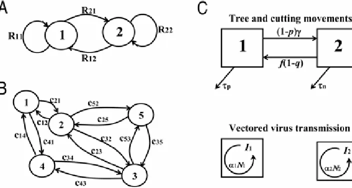
(i = 1,2) resulting from one mother lesion on cultivar j (j = 1,2), which we will denote by Rij (Fig. 2A). That is, new lesions on a given cultivar have been caused by previously existing lesions on either cultivar. For example, to calculate R11, one should realize
that the total number of spores produced by a lesion on cultivar 1 equals α1τ1, a fraction ρqH of these spores is deposited on a leaf
of cultivar 1, and a fraction γ1 of these deposited spores germinates
and forms a daughter lesion. Therefore R11 = γ1α1τ1ρqH. Similar
reasoning gives R22 = γ2α2τ2ρ(1 – q)H, R21 = γ2α1τ1ρ(1 – q)H, and
R12 = γ1α2τ2ρqH. Note that the latter two expressions account for
Fig. 1. The density of lesions, In, as a function of the pathogen generations, n, elapsed since the start of the experiment for three values of the basic reproduction number, R0. Left graph, ordinary scale; right graph, log-scale.
new lesions developing on the ‘opposite’ cultivar to the one where the spores were produced.
Using these four elements we build a model for the dynamics of the lesion density on leaves of cultivar 1 in generation n, I1,n,
and on cultivar 2, I2,n. If there are I1,n lesions on cultivar 1 in
generation n these lesions will cause R11I1,n lesions on cultivar 1 in
generation n+1. Similarly I2,n lesions on cultivar 2 will cause R12I2,n lesions on cultivar 1 in pathogen-generation n+1. Our
model equation relating lesion numbers in successive pathogen-generations on cultivar 1 thus reads I1,n+1= R11I1,n + R12I2,n. Similar
arguments can be used to derive the model equation for lesion numbers on cultivar 2. Our model for the development of lesion numbers thus reads
I1,n+1= R11I1,n + R12I2,n
I2,n+1= R21I1,n + R22I2,n (3)
A more compact notation of such models is the matrix-vector notation
n n AI
Ir+1= r (4)
where
⎟⎟ ⎠ ⎞ ⎜⎜ ⎝ ⎛ =
,n ,n n
I I I
2 1
r
and ⎟⎟
⎠ ⎞ ⎜⎜
⎝ ⎛ =
22 21
12 11
R R
R R
A (5)
Some further information about matrix vector notation can be found in, for example, the books by Bretcher (3) and Caswell (4, pages 652-668).
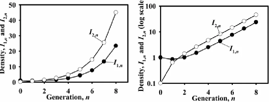
The model can be solved numerically in the same way as we solved equation 1. Figure 3 shows results for a specific set of parameter values and initial conditions. These graphs show that, exactly as for equation 1, the density of lesions on each of the cultivars increases from generation to generation, with a constant multiplication factor. This increase is the same factor for I1 and I2
(see Discussion) after a few generations. The deviation from this pattern for the first few generations, in this specific case n < 3, is due to the chosen initial conditions, whose influence quickly disappears. The multiplication factor, λd, is calculated from λd =
Ii,n+1/Ii,n (i = 1,2) for non-small values of n, so that the influence of
the initial conditions does not affect λd. Now note that since our
model has a time step of one generation, λd is the
generation-to-generation multiplication factor and is thus the basic reproduction number, R0.
We conclude that the recipe in the previous section also applies to model equations 3, but that the multiplication factor has to be calculated at values of n for which the effects of the initial condi-tion have disappeared. Box 2 gives some elaboracondi-tions of the re-sults of this example using the numerical recipe. In the
Discus-sion, we explain in more detail why the solutions are affected by the initial conditions for small values of n.
Models of the structure of equation 4 can be solved analytically (2–4). Given the results above and Figure 3, for large values of n
it is not surprising that the solutions are given by
2 , 2
1 , 1
C I
C I
n d n
n d n
λ =
λ =
(6)
where the constants C1 and C2 are related to the initial densities of
infection. The λd can directly be calculated from matrix A in
equation 4 (3,4,12), and is called the dominant eigenvalue of A, which is
(
)
(
)
2
4 11 22 21 12 2
22 11 22
11 R R R R R R R
R + + + − −
=
λ (7)
Substituting the expressions for Rij and some algebraic manipu-lation we find that
(
H)
q(
H)
q
R0= γ1α1τ1ρ +(1− )γ2α2τ2ρ (8)
Equation 6 shows that the dominant eigenvalue is the growth factor for the density of lesions in each time step. Since the time step equals one generation, this dominant eigenvalue is the gen-eration-to-generation multiplication factor and thus the basic reproduction number.
Box 2 gives some notes on and elaborations of this expression. Note that in cases where the matrix is larger than 2 × 2, analytical solutions for the eigenvalue are not generally available, except in very special cases; however, algorithms for finding them are included in many statistical and mathematical packages, as well as in some spread-sheet programs (Appendix).
For two-component systems, we can state that (as illustrated here) the model for the generation-to-generation dynamics of lesion density can be used to calculate R0. Subsequently, the
ex-pression for R0 can be used to study the effect of parameter values
(relating to the process under study, such as infectious period and sporulation rate) on the basic reproduction number, either numerically or explicitly using equations 7 and 8.
Note on the assumption of negligible duration of the latent period. The method described above is easily extended to include nonnegligible duration of the latent period. Each of the matrix entries Rij then needs to take account of the probability that a lesion survives through the latent period and enters the infectious period. In many models for animal and human pathogens, this probability equals 1, for plant pathogens, however, the probability to survive the latent period can be less than 1, for example due to plant defense responses and/or leaf necrosis/leaf shedding.
Fig. 3. Pathogen dynamics in a cultivar mixture. The density of lesions on cultivar 1, I1,n, and on cultivar 2, I2,n, as a function of the pathogen generations, n, elapsed since the start of the epidemic. These are calculated using equation 3, with parameter values R11=0.8, R12 = 0.5, R21 = 0.5, R22 = 1.5, and initial conditions
Throughout the paper we assume a negligible duration of the latent period because this simplifies the presentation. We note however again that extensions to include a nonnegligible latent period duration are easily done.
EXAMPLE 2: PATHOGEN DISPERSAL IN A LANDSCAPE
Consider a soilborne pathogen invading a system of fields in a region. The pathogen is dispersed between fields in soil on tractor wheels, farmer boots, etc. As a specific example, one can think of the invasion of Polymyxa betae, a soilborne protist that infects fibrous roots of sugar beet plants. The pathogen itself does not cause major damage, but the virus it transmits, Beet necrotic yellow vein virus (BNYVV), does cause severe damage to sugar beet crops (2,17,31,35,38).Assume we are interested in the effect of the spatial arrangement of the fields in the region on R0. For the
sake of simplicity here (although the approach is easily general-ized), we assume that all fields are identical and that dispersal depends only on the distance between fields. We model the
density of infected plants, Ii,n, in each field i in generation n. The
epidemic conditions are as follow.
• Each infected plant produces α infectious propagules per time unit.
• A fraction d of these infectious propagules is dispersed in soil on tractor wheels and farmer boots.
• An infectious propagule is dispersed from field j to field i
with probability cij; cij will be called the connectivity be-tween field j and field i.
• An infectious unit has a probability γH to infect a plant, where H is the crop density and γ the infection parameter.
• A plant is infectious for τ time units.
Consider an infected plant in field 1, and assume here there are five fields. During its entire infectious period this plant produces
ατ infectious propagules, of which a fraction 1 – d stays in field 1; thus, in the next generation, each infection causes γH(1 – d)ατ daughter infections. A fraction d is dispersed, and of these pro-pagules, a fraction c21 reaches field 2. The total number of
the same reasoning for the assemblage of fields shown in Figure 2B, where no arrows between fields means no dispersal, we find the model equations:
n n n n n n n n n n n n n n n n n n n n n n n n n n n n n n I d H I Hdc I Hdc I Hdc I Hdc I I Hdc I d H I Hdc I Hdc I Hdc I I Hdc I Hdc I d H I Hdc I Hdc I I Hdc I Hdc I Hdc I d H I Hdc I I Hdc I Hdc I Hdc I Hdc I d H I , 5 , 4 54 , 3 53 , 2 52 , 1 51 1 , 5 , 5 45 , 4 , 3 43 , 2 42 , 1 41 1 , 4 , 5 35 , 4 34 , 3 , 2 32 , 1 31 1 , 3 , 5 25 , 4 24 , 3 23 , 2 , 1 21 1 , 2 , 5 15 , 4 14 , 3 13 , 2 12 , 1 1 , 1 ) 1 ( ) 1 ( ) 1 ( ) 1 ( ) 1 ( ατ − γ + ατ γ + ατ γ + ατ γ + ατ γ = ατ γ + ατ − γ + ατ γ + ατ γ + ατ γ = ατ γ + ατ γ + ατ − γ + ατ γ + ατ γ = ατ γ + ατ γ + ατ γ + ατ − γ + ατ γ = ατ γ + ατ γ + ατ γ + ατ γ + ατ − γ = + + + + + (9)
or in matrix vector notation In In
r r
A 1=
+ , where
⎟⎟ ⎟ ⎟ ⎟ ⎟ ⎟ ⎠ ⎞ ⎜⎜ ⎜ ⎜ ⎜ ⎜ ⎜ ⎝ ⎛ = n n n n n n I I I I I I , 5 , 4 , 3 , 2 , 1 r ⎟ ⎟ ⎟ ⎟ ⎟ ⎟ ⎠ ⎞ ⎜ ⎜ ⎜ ⎜ ⎜ ⎜ ⎝ ⎛ ατ − γ ατ γ ατ γ ατ γ ατ γ ατ γ ατ − γ ατ γ ατ γ ατ γ ατ γ ατ γ ατ − γ ατ γ ατ γ ατ γ ατ γ ατ γ ατ − γ ατ γ ατ γ ατ γ ατ γ ατ γ ατ − γ = ) 1 ( ) 1 ( ) 1 ( ) 1 ( ) 1 ( 54 53 52 51 45 43 42 41 35 34 32 31 25 24 23 21 15 14 13 12 d H c Hd c Hd c Hd c Hd c Hd d H c Hd c Hd c Hd c Hd c Hd d H c Hd c Hd c Hd c Hd c Hd d H c Hd c Hd c Hd c Hd c Hd d H A (10)
Finally, we calculate R0 by numerically solving model equation 9
and, for large values of n, calculate R0 = Ii,n+1/Ii,n. Box 3 gives
some elaborations of this example.
As mentioned above, in principle, R0 can be determined
analytically as the dominant (first) eigenvalue of the 5 × 5 matrix
A in equation 10. Despite the fact that, no simple formula exists, in general, for the eigenvalues of 5 × 5 matrices, the dominant eigenvalue can be easily calculated with the use of a mathematical software package. This avoids the necessity of performing the tedious exercise of (i) numerically solving the model system in equation 9, (ii) looking through the output to determine when the effects of the initial conditions on disease dynamics have dis-appeared, and (iii) calculating R0 for pairs of generations. The
to the dominant eigenvalue can be developed, as exemplified in Box 3.
EXAMPLE 3: PROPAGATOR TREES AND NURSERIES: COPING WITH TYPE CHANGE
Introduction.We first generalize our terminology and call an Ij
plant in examples 1 and 2 ‘an individual of type j’. That is, in example 1, a type 1 individual is a lesion on a plant of cultivar 1, and in example 2, it is an infected plant in field 1. In both ex-amples infected plants do not change type during their infectious period. An infected plant of cultivar 1 (or in field 1) remains so during its entire infectious period. Obviously there are many circumstances in which infected individuals can change type. For example, garden plants are often grown in a nursery, then dis-tributed to garden centers and subsequently sold for planting in homeowner gardens. A plant that becomes infected in the nursery (a type 1, I1, individual) changes type when transported to a
garden center (and becomes a type 2, I2, individual), and changes
type again (into type 3, I3) when sold to a garden owner.
We introduce a system with one type-change and derive the equations for this specific example. Next we generalize and allow for any type change to occur. We will see that this generalization actually simplifies the model derivation through the introduction of a matrix describing the pathogen transmission rates from type j to type i, and a matrix describing the amount of time an individual in-fected while type j spends being type i during its infectious period.
The special example. Fruit trees, such as plum, are multiplied by taking cuttings from propagator trees and growing them for some time in a nursery. The majority of the established cuttings are sold to orchard/garden owners, and a small fraction is used to establish new propagator trees. We consider here, as an example, the pathogen Plum pox virus (PPV), a member of the genus
Potyvirus, causing plum pox disease (Sharka) in plum and some other tree species (5,25). This virus is transmitted by aphids and through cuttings taken from infected propagator trees.
Denote the density of infected propagator trees in generation n
by I1,n and the density of infected cuttings in the nursery by I2,n.
The ‘type change’ that occurs in this system is that individuals of type 2 can change into individuals of type 1, when they are used to establish a new propagator tree. The life-cycle components in this pathosystem are (Fig. 2C) as follows.
• Cuttings stay τc time units in the nursery, after which a
fraction f is used to establish new propagator trees. The remaining fraction, 1 – f, is sold to orchards/garden owners.
• Before selling or being used as new propagator trees, the cuttings are screened and an infected tree is detected and discarded with probability q.
• A propagator tree is used for τp time units and then removed.
• In each time unit, γ cuttings are taken from each propagator tree.
• Before planting in the nursery the cuttings are screened and infected cuttings are detected and discarded with prob-ability p.
• Due to insect-vectored transmission, an infected propagator tree causes α1N1 new infected propagator trees per time
unit, where N1 is the density of healthy propagator trees
and α1 is the transmission coefficient.
• Due to vectored transmission, an infected cutting in the nursery causes α2N2 new infected cuttings in the nursery
per time unit, where N2 is the density of healthy cuttings in
the nursery and α2 is the transmission coefficient.
We refer to equations 3, 4, and 5 for the model structure, and develop the matrix elements Rij. To this end, we follow a freshly infected propagator tree and calculate how many daughter infec-tions it causes in the field with propagator trees and in the nursery during its entire infectious period; the process is repeated for a freshly infected cutting in the nursery.
• An infected propagator tree causes α1N1 new infected
propagator trees per time unit and does this for τp time
units giving R11 = α1N1τp. From an infected propagator tree,
cuttings are taken (per time unit) and after screening, a fraction (1 – p) is planted in the nursery. This is done for τp
time units giving R21 = (1 – p)γτp for infections in the
nursery arising from infected propagator trees.
• An infected cutting in the nursery causes α2N2 new infected
cuttings per time unit and does this for τn time units, giving
a total of α2N2τc daughter infections. In addition, after screening, a fraction, f(1 – q), of the infected cuttings changes type by being used to establish new propagator trees, and from these propagator trees (1 – p)γτp infected
cuttings are taken and planted in the nursery. The two sources of infected cuttings together give us R22= α2N2τc +
f(1 – q)(1 – p)γτp. Note that the (1 – p)γτp term of R22is the
same as R21.
• For the final matrix element, R12, the multiplication factor
for infected propagator plants arising from infected nursery plants, again realize that a cutting is used to establish a new propagator tree with probability f(1 – q), and that an in-fected propagator tree causes α1N1τp new infected
propa-gator trees. This gives us R12= f(1 – q) α1N1τp.
The matrix A in equation 5 thus has the form
⎟⎟ ⎠ ⎞ ⎜⎜ ⎝ ⎛ τ − γ − + τ α γτ − τ − α τ α = p c p p p A ) 1 ( ) 1 ( ) 1 ( ) 1 ( 2 2 1 1 1 1 q f p N p q f N N (11)
and the basic reproduction number can be calculated by substi-tuting the matrix elements in equation 6. Box 4 discusses the effect of disease control efforts in the propagator trees and in the nursery on the basic reproduction number.
Generalization. The two matrix components affected by type change of infected cuttings in the nursery into infected propagator trees are R12 and R22, the top right and bottom right element of the
matrix, respectively. First consider R12. As required, the
dimen-sion of R12 is number (i.e., number of new infected individuals of
type 1 arising from infected individuals of type 2) because the parameter combination α1N1 is a rate (number of new infections
per time unit) and it is multiplied by f(1 – q)τp, which has the
dimension of time. What exactly is the interpretation of f(1 –
q)τp? The term relates to infected cuttings in the nursery that
change type and become infected propagator trees. A fraction f(1 –
q) of the infected cuttings actually change type, the others, 1 – f(1 –
q), are removed (sold or detected infected) from the system. One could say that this last group spends 0 time units as an infected propagator tree and the first group spends τp time units as infected
propagator trees. This means that, on average, an infected cutting in the nursery will change type and spend 0⋅(1 – f(1 – q)) + τpf(1 –
p) = τpf(1 – q) time units as an infected propagator tree. We can
thus write
12 11
12 r T
2 type being infected became individual the when 1 type as spent time of amount 1 type of individual an from 1 type of unit time per infections new of number R = ⎥ ⎥ ⎥ ⎦ ⎤ ⎢ ⎢ ⎢ ⎣ ⎡ • ⎥ ⎥ ⎥ ⎦ ⎤ ⎢ ⎢ ⎢ ⎣ ⎡
= (12)
The matrix element R22 has a similar structure with α1N1 and (1 –
p)γ being rates (vectored transmission between cuttings within the nursery and vertical transmission with cuttings taken from propagator trees) and τc and f(1 – q)τp being time units. This term
can thus be interpreted as
In the most general case, all possible pathogen transmissions between types and all possible type-changes would be possible. In that case, we can define: rij as the number of infected individuals of type i caused by infected individuals of type j, per time unit; and Tij as the amount of time an individual that became infected being type j spends being infectious as type i. We can then write
⎟⎟ ⎠ ⎞ ⎜⎜
⎝ ⎛
+ +
+ +
=
12 21 22 22 21 22 11 21
22 12 12 11 21 12 11 11
T r T r T r T r
T r T r T r T r
A (14)
In general, equation 14 is not necessarily directly intuitive, but its structure can be derived by considering each term individually and constructing the equation from the logical interconnection of terms. For the specific example, some of the terms are zero, for example r12 equals zero because cuttings in the nursery do not
infect propagator trees via vectored disease transmission and T21
equals zero because propagator trees do not change type (i.e., they are not transferred to a nursery).
Readers familiar with matrix multiplication will recognize that equation 14 can be written as
⎟⎟ ⎠ ⎞ ⎜⎜ ⎝ ⎛ ⎟⎟ ⎠ ⎞ ⎜⎜ ⎝ ⎛ =
22 21
12 11
22 21
12 11
T T
T T r r
r r
A (15)
Equation 15 can also be written in the more compact form A =
RT, with R and T denoting the matrices of rates and times, respectively. Readers not familiar with matrix multiplication can either take equations 14 and 15 as defining matrix multiplication or consult, for example, the books by Bretcher (3) and Caswell (4) or any other text book about linear algebra. Developing a model to calculate the basic reproduction number is, thus, using equation 15, a matter of finding expressions for all rij and Tij in terms of the life-cycle components of the pathogen in the pathosystem under consideration. Equations 14 and 15 of course generalize to systems with three or more types.
DISCUSSION
The value of R0in understanding and quantifying population
dis-ease control strategies to R0, utilization of this metric has remained
uncommon in plant disease epidemiology, apart from several exceptions. Models formulated in terms of nonlinear differential equations are useful for many purposes, but as demonstrated in Box 1, thresholds derived for epidemics from such models may not, in fact, be equivalent to R0. For simple systems (e.g., one host
population, one pathogen strain), it is relatively straightforward to derive an expression for R0 based on first principles (27).
How-ever, for more complex systems, such derivations also become complex. The methods originally developed by Diekmann et al. (8) and Heesterbeek (16) provide the framework for dealing with complexity of pathosystems in the derivation of the metric.
In this paper, we built on the work of Diekmann and Heesterbeek to derive R0for several complex scenarios of relevance in plant
pathology. We need to stress that the methods introduced in this paper are not meant to be a means of simulating epidemic progress curves. The only reason we showed some epidemic progress curves (Figs. 1 and 3), and discussed the curves, was to help make a convincing argument of how to calculate R0 from a
model that has the time step of a pathogen generation. We encourage investigators to apply the matrix methods to obtain R0
by either using one of the computer programs discussed in the Appendix, or in the 2 × 2 case, to calculate the largest eigenvalue of the matrix (which then equals R0), by using equation 7.
In most applications of the methods, the final step will be to plot graphs of R0 as a function of life-cycle parameters. This can
only be done by assigning numerical values to all parameters in the model. This implies that these parameter values need to be estimated from published or unpublished data. While parameter estimation is an important topic and potentially challenging in practice, it is outside the scope of this paper. Some of the methods that are used are introduced in Madden et al. (27), where refer-ences for further reading are suggested. Caswell (4) and the literature cited therein provide a good introduction to the issues of estimation for life cycle parameters in matrix models.
Several issues related to the applicability of the methodology in this paper, not discussed so far in an effort to avoid unnecessary complexity, are covered individually below. First, the methods apply to pathogens with discrete generations as well as to patho-gens with overlapping generations. Although the methods using matrix approaches introduced in this paper use the pathogen generation time as basic time step, they are not only applicable to pathogens with generations that are separated in time (so that at each point in time only one generation of the pathogen is alive or active). The methods are equally well applicable to pathogens where a (large) number of generations occur in overlapping time-windows. This follows from the general theory (8). Recall that R0
is the number of secondary infections from one mother infection at infinitesimally low pathogen density. At such low densities, so-called density-dependent interactions between pathogen indivi-duals (e.g., lesions) are negligible. Thus, each pathogen individual produces offspring without any interaction with other pathogen individuals, and the sum of the number of offspring produced is not affected by whether the pathogen generations are separated in time or overlapping.
Second,formulation of the matrix on a generation-to-genera-tion basis is essential for proper derivageneration-to-genera-tion of R0. It is very
important to bear in mind that we have been able to equate the largest eigenvalue of the matrix A to R0 because the time step in
the models was the same as the generation time. If a model is constructed that calculates the densities of infected individuals in the various categories using a time step not equal to the patho-gen’s generation time, the largest eigenvalue of the matrix does measure the growth of the population over the time step, but the eigenvalue is not equal to R0.
Third, although matrices have more than one eigenvalue the largest eigenvalue is the basic reproduction number, R0. Solutions
of models of the form of equations 3 and 4 and 9 and 10 are sums
of terms of the form of equation 6. For example the full solution of equation 3 is
n n d n
n n d n
C C I
C C I
2 4 2 , 2
2 3 1 , 1
λ + λ =
λ + λ =
(16)
where λd is the largest eigenvalue of A and is given by equation 7,
and λ2 is the other eigenvalue of this matrix and is given by
equation 7 when we replace the + sign in the square root by a – sign. The λd components of this solution grow faster than the
λ2components and therefore for larger values of n the
contribu-tion of λ2 is negligible, leading to the conclusion that λd is the
generation to generation multiplication factor. The contribution to the solution of the eigenvalue λ2 causes the deviations at small n
as discussed above. (For those familiar with complex eigenvalues: the largest eigenvalue will always be real because the number of offspring cannot be a complex number.)
Fourth,multiple infection transformations are not a component of the basic reproduction number. The above mentioned infinite-simally low pathogen density has another effect on methods sim-plifying the construction of the model to calculate R0. Consider a
lesion-forming, spore-producing, fungal leaf pathogen. At in-finitesimally low pathogen density, the probability that a spore lands on an existing lesion is negligible, and thus its probability to germinate, infect, and form a lesion is not affected by other lesions. Thus, no corrections are needed for the build-up (in-crease) in density of infections. Besides the use of R0 as a
gen-eration to gengen-eration multiplication factor, it also has some uses in situations where density dependence does play a role. In many models (but not all!), R0can be used to determine the ultimate or
steady-state value of disease or pathogen density in a host population (10,21,23,26,27,34).
Fifth, initial conditions do not affect R0. As we have shown
from the numerical approach (Fig. 3), the density of the various types of infected individuals can increase or decrease in the first few generations, depending on the initial conditions. This is be-cause the early population dynamics depend on the initial (i.e., in generation n = 0) density of individuals in different categories and on the matrix structure. However, R0 determines whether in the
long run the pathogen density will increase, R0> 1, or the
patho-gen will die out, R0< 1. In other words, R0 is only dependent on
the matrix structure and not on the initial conditions (i.e., R0 is
defined strictly from the matrix of parameters and not from the initial conditions involving infection density).
Sixth,R0is a number and not a rate, by definition. However, it
might be confusing to see in, for example, Caswell’s book that the largest eigenvalue (λd) is often called the “population growth rate”
(4). The models Caswell discusses usually have time steps of a length other than the generation time of the organism under consideration. In the methods explained in this paper, the time step is one generation and the largest eigenvalue measures the growth of the density of infected individuals per this generation step. This choice of time step provides the direct link between the largest eigenvalue and the generation-to-generation multiplica-tions factor, R0 (a number).
To conclude, the aim of this paper was to translate some of the existing mathematical framework (8) for the calculation of R0 into
a language palatable to plant epidemiologists. The key reason for this is that using the framework, it is possible to calculate R0 in a
relatively simple way based on a description of the life-cycle components and the interactions with the host in complex situa-tions. Virtually any level of detail deemed necessary for the specific case under consideration can be incorporated in the approach. In contrast, the calculation of R0 for such complex
situations from a model formulated as a set of nonlinear differ-ential (or difference) equations can easily lead to a threshold expression which is not equal to R0. Although nonlinear
APPENDIX
Numerical recipes to calculate the dominant eigenvalue.
This appendix provides programming scripts for finding the dominant or maximum eigenvalue of an n ×n matrix and some other software tips for starting to use matrix projection models. Scripts are available for several commonly used programming languages.
The specific numerical values of the matrix entries used in this appendix do not relate to the examples discussed in the main text. They are only given so that the reader can check whether he/she finds the correct eigenvalue when using one of the programs.
Excel. The data analysis tools included in Excel do not include eigenvalue calculations. However, a number of freeware and commercial add-ins to Excel do include these functions. Here we highlight one of these which has been developed specifically to add tools for matrix population modeling to Excel. This is the PopTools add-in developed by Greg Hood at CSIRO, Australia. Instructions for obtaining and installing PopTools can be found at http://www.cse.csiro.au/poptools/. Once PopTools is loaded, an extra menu item appears on the Excel menu bar allowing the user to call the various Poptools functions. The steps required to obtain the value of R0 are as follow.
1. Enter the values of the projection matrix into a suitable n × n grid of cells.
2. Highlight the matrix.
3. From the PopTools menu choose Matrix tools: eigen-analysis (symmetric).
4. A dialogue box appears with the cell range specifying the matrix already entered.
5. Enter a suitable cell reference for the output. 6. Click Go.
7. The eigenvalues and eigenvectors for the matrix will be entered into the worksheet. The eigenvectors are printed on the left in an n × n block. The eigenvalues are printed on the right of the output with a different cell background color. The eigenvalues are printed in descending order; the first one is the estimated value of R0.
Mathcad template. Although Mathcad includes programming controls, its user interface is in the form of a WYSWIG mathematics notebook. The steps required to obtain the value of R0 are as follows.
1. Define the projection matrix, A, containing the multipli-cation and transfer rates.
⎟⎟ ⎠ ⎞ ⎜⎜
⎝ ⎛ =
075 . 1 05 . 0
05 . 0 1 . 1 :
A
2. Use the built in “eigenvals” function to get the numerical values of the eigenvalues of A.
A) eigenvals(
A =
λ :
3. Print the eigenvalues of A by using the = key.
4. Mathcad automatically sorts the eigenvalues with the largest first.
⎟⎟ ⎠ ⎞ ⎜⎜ ⎝ ⎛ = λ
036 . 1
139 . 1 A
MATLAB script. The code given below can either be run directly as separate lines or in its entirety when collated into an .m file. Note that the file name cannot contain spaces. The steps required to obtain the value of R0 are as follows.
1. Define matrix, A. The letters within the matrix structure represent the matrix elements, whereby matrix rows are separated by “;”.
A = [a b c ; ...
d e f ; ...
g h i ];
2. Calculate the eigenvalues of A and store them in “lambda”
lambda = eig(A)
3. Determine the number of elements in vector “lambda”
[a,b] = size(lambda)
4. Determine which elements of “lambda” are noncomplex and return 1 to “NonComplex” if the element is not com-plex and 0 when the element is comcom-plex
for i = 1:a
NonComplex(i) = isreal(lambda(i)) end
5. Determine the maximum real eigenvalue
MaxLambda = max(NonComplex'.*lambda)
ACKNOWLEDGMENTS
F. van den Bosch thanks DEFRA for financial support of the project “Development and testing of a model epidemiological framework to optimize the detection and intervention strategies for plant pathogens of statutory concern.’’ Rothamsted research received support from the Biotechnology and Biological Research Council (BBSRC) of the United Kingdom. F. van den Bosch thanks H. “R0” Heesterbeek for useful discussions on the basic reproduction number. Scottish Agricultural College received financial support from the Scottish Executive Environment and Rural Affairs Department. Ohio State University received funding from state and federal agencies.
LITERATURE CITED
1. Adler, F. R., and Nuernberger, B. 1994. Persistence in patchy irregular landscapes. Theor. Popul. Biol. 45:41-75.
2. Asher, M. J. C. 1993. Rhizomania. Pages 313-346 in: The Sugar Beet Crop: Science Into Practice. D. Cooke and R. Scott, eds. Chapman and Hall, London, UK.
3. Bretcher, O. 1997. Linear Algebra with Applications. Prentice Hall, Upper Saddle River, NJ.
4. Caswell, H. 2001. Matrix Population Models. 2nd ed. Sinauer Associates, Inc. Publishers. Sunderland, MA.
5. Chan, M.-S., and Jeger, M. J. 1994. An analytical model of plant virus disease dynamics with rouging and replanting. J. Appl. Ecol. 31:413-427. 6. De Jong, M. C. M., Diekmann, O., and Heesterbeek, J. A. P. 1994. The
computation of R0 for discrete-time epidemic models with dynamic heterogeneity. Math. Biosci. 119:97-114.
7. de Koeijer, A., Heesterbeek, H., Schreuder, B., Oberthur, R., Wilesmith, J., van Roermund, H., and de Jong, M. 2004. Quantifying BSE control by calculating the basic reproduction ratio R-0 for the infection among cattle. J. Math. Biol. 48:1-22.
8. Diekmann, O., Heesterbeek, J. A. P., and Metz, J. A. J. 1990. On the definition and the computation of the basic reproduction ratio R0 in models for infectious-diseases in heterogeneous populations. J. Math. Biol. 28:365-382.
9. Diekmann, O., Dietz, K., and Heesterbeek, J. A. P. 1991. The basic reproduction ratio for sexually-transmitted diseases. 1. Theoretical considerations. Math. Biosci. 107:325-339.
10. Diekmann, O., and Heesterbeek, J. A. P. 2000. Mathematical Epidemiology of Infectious Diseases. Model Bulding, Analysis and Interpretation. John Wiley & Sons, Chichester, England.
11. Dietz, K., Heesterbeek, J. A. P., and Tudor, D. W. 1993. The basic reproduction ratio for sexually-transmitted diseases 2. Effects of variable HIV infectivity. Math. Biosci. 117:35-47.
12. Edelstein-Keshet, L. 2005. Mathematical Models in Biology. Society for Industrial and Applied Mathematics, Philadelphia.
13. Gilligan, C. A. 2002. An epidemiological framework for disease management. Adv. Bot. Res.38:1-64.
14. Gubbins, S., Gilligan, C. A., and Kleczkowski, A. 2000. Thresholds for invasion in plant-parasite systems. Theor. Popul. Biol.57:219-234. 15. Gubbins, S., and Gilligan, C. A. 1999. Invasion thresholds for fungicide
resistance. Proc. R. Soc. Ser. B 266:2539-2549.
16. Heesterbeek, J. A. P. 2002. A brief history of R-0 and a recipe for its calculation. Acta Biotheor. 50:375-376.
17. Heijbroek, W. 1988. Dissemination of rhizomania by soil, beet seeds and stable manure. Neth. J. Plant Pathol. 94:9-15.
18. Jackson, D. I., and Looney, N. E. 1999. Temperate and suptropical fruit production. CABI Publishing, Wallingford, UK.
20. Jeger, M. J., Jones, D. G., and Griffiths, E. 1981. Disease progress of non-specialized fungal pathogens in intraspecific mixed stands of cereal cultivars. II. Field experiments. Ann. Appl. Biol. 98:199-210.
21. Jeger, M. J., and van den Bosch, F. 1994. Threshold criteria for model plant disease epidemics. I. Asymptotic results. Phytopathology 84:24-27. 22. Jeger, M. J., van den Bosch, F., and Dutmer, M. Y. 2002. Modeling plant
virus epidemics in a field-nursery system. IMA J. Math. Appl. Med. 19:75-94.
23. Kermack, W. O., and McKendrick, A. G. 1927. A contribution to the mathematical theory of epidemics. Proc. R. Soc. Lond. Ser. A 115:700-721.
24. Lamb, K., Kelly, J., and Bowbrick, P. 1995. Nursery stock Manual. Growers Manual No. 1. 2nd ed. Grower Books, Nexus Media Limited, Kent.
25. Levy, L., Damsteegt, V., Scorza, R., and Kolber, M. 2000. Plum Pox Potyvirus Disease of Stone Fruits. APSnet Feature. Published online by The American Phytopathological Society, St. Paul, MN.
26. Madden, L. V., and van den Bosch, F. 2002. A population-dynamics approach to assess the threat of plant pathogens as biological weapons against annual crops. BioScience 52:65-74.
27. Madden, L. V., Hughes, G., and van den Bosch, F. 2007. The Study of Plant Disease Epidemics American Phytopathological Society, St. Paul, MN.
28. Madden, L. V., Jeger, M. J., and van den Bosch, F. 2000. A theoretical
assessment of the effects of vector-virus transmission mechanisms on plant virus disease epidemics. Phytopathology 90:576-594.
29. Mundt, C. C. 2002. Use of multiline cultivars and cultivar mixtures for disease management. Annu. Rev. Phytopathol. 40:381-410.
30. Park, A. W., Gubbins, S., and Gilligan, C. A. 2001. Invasion and persistence of disease in a spatially structured metapopulation. Oikos 94:162-174.
31. Richard-Molard, M. 1985. Rhizomania: A world-wide danger to sugar beet. Span 28:92-94.
32. Roberts, M. G., and Heesterbeek, J. A. P. 2003. A new method for estimating the effort required to control an infectious disease. P. Roy. Soc. Lond. B-Bio. 270:1359-1364.
33. Ross, R. 1911. The Prevention of Malaria. 2nd ed. Murray, London. 34. Segarra, J., Jeger, M. J., and van den Bosch, F. 2001. Epidemic dynamics
and patterns of plant diseases. Phytopathology 91:1001-1010.
35. Stacey, A. J., Truscott, J. E., Asher, M. J. C., and Gilligan, C. A. 2004. A model for the invasion and spread of Rhizomania in the United Kingdom: Implications for disease control strategies. Phytopathology 94:209-215. 36. Vanderplank, J. E. 1963. Plant Diseases: Epidemics and Control.
Academic Press, NY.
37. Vanderplank, J. E. 1975. Principles of Plant Infection. Academic Press, New York.