University of New Orleans University of New Orleans
ScholarWorks@UNO
ScholarWorks@UNO
University of New Orleans Theses and
Dissertations Dissertations and Theses
Summer 8-10-2016
Experimental Study and Numerical Simulation of Methane Oxygen
Experimental Study and Numerical Simulation of Methane Oxygen
Combustion inside a Low Pressure Rocket Motor
Combustion inside a Low Pressure Rocket Motor
mine kaya
University of New Orleans, [email protected]
Follow this and additional works at: https://scholarworks.uno.edu/td
Part of the Heat Transfer, Combustion Commons
Recommended Citation Recommended Citation
kaya, mine, "Experimental Study and Numerical Simulation of Methane Oxygen Combustion inside a Low Pressure Rocket Motor" (2016). University of New Orleans Theses and Dissertations. 2240.
https://scholarworks.uno.edu/td/2240
This Thesis-Restricted is protected by copyright and/or related rights. It has been brought to you by
ScholarWorks@UNO with permission from the rights-holder(s). You are free to use this Thesis-Restricted in any way that is permitted by the copyright and related rights legislation that applies to your use. For other uses you need to obtain permission from the rights-holder(s) directly, unless additional rights are indicated by a Creative Commons license in the record and/or on the work itself.
Experimental Study and Numerical Simulation of Methane Oxygen Combustion inside a Low Pressure Rocket Motor
A Thesis
Submitted to the Graduate faculty of University of New Orleans
in partial fulfillment of the requirements for the degree of
Master of Science In
Mechanical Engineering Thermal Fluids Science
by
Mine Kaya
B.Sc., Middle East Technical University, 2012
ii
iii
iv
Acknowledgements
First of all, I would like to emphasize the contribution from my supervisor Dr. Kazim M.
Akyuzlu. This work would not have been accomplished without his invaluable guidance and
encouragement. I would also like to thank Dr. Martin J. Guillot, Dr. Paul Herrington and Dr.
Paul Schilling for serving on my thesis committee.
I am grateful to my classmates Seda, Amer and Jose for their friendship, encouragement and
help throughout this year.
This research was supported in part by NASA EPSCoR and Board of Regents Support Fund /
v
TABLE OF CONTENTS
NOMENCLATURE ... vii
TABLE OF TABLES ... ix
TABLE OF FIGURES ... x
ABSTRACT ... xii
1. INTRODUCTION ... 1
2. LITERATURE SURVEY ... 2
3. DESCRIPTION OF PHYSICAL MODEL ... 3
4. EXPERIMENTAL STUDY... 6
4.1. Description of the Experimental Setup ... 6
4.2. Experimental Procedure and Operating Conditions ... 9
4.3. Data Analysis ... 10
5. NUMERICAL STUDY ... 11
5.1. Mathematical Formulation ... 11
5.2. Solution Technique ... 16
6. RESULTS ... 18
6.1. Results of the Experiments ... 18
6.2. Results of the Computational Model ... 23
6.2.1. Validation of Computational Model ... 24
6.2.2. Grid Independence Study ... 28
6.3. Comparison of Computational and Experimental Results ... 41
6.4. Parametric Study ... 46
6.4.1. Effect of Different Mass Flow Rates ... 46
6.4.2. Effect of Different Outlet Pressures ... 50
7. CONCLUSIONS... 52
8. RECOMMENDATIONS ... 54
REFERENCES ... 55
APPENDICES I. EQUIPMENT LIST USED IN THE EXPERIMENTS………..57
II. CALIBRATION CURVES FOR THE EXPERIMENTS………..58
III. CALCULATION OF THE FUEL MASS FLOW RATE………..61
IV. VECTOR FORM OF THE GOVERNING DIFFERENTIAL EQUATIONS...62
V. LOG SHEETS OF THE EXPERIMENTS……….63
VI. RESULTS OF RUN 2……….65
VII.PARAMETERS FOR THE BASE CASE (CCNF-R-I) SIMULATION………67
vi
NOMENCLATURE
Symbols
A Absorption coefficient
A Empirical constant
Ar Pre-exponential factor
B Empirical constant
C Constant, molar concentration
cp Specific heat
D Diffusion coefficient, energy transfer due to species diffusion
Er Activation energy
G Incident radiation
J Diffusion flux of species
K Thermal conductivity, turbulent kinetic energy
kf Arrhenius rate
M Molecular mass
N Refractive index
P Pressure
Pr Prandtl number
R Production rate of species
R Universal gas constant
S Modulus of the mean rate of strain tensor
Sc Schmidt number
T Time
T Temperature
U Velocity in x direction
V Velocity in y direction
V Velocity
vii Greek Symbols
Ε Turbulence dissipation rate
Η Rate exponent
Μ Viscosity
Ν Stoichiometric coefficient
Φ Viscous dissipation
Ρ Density
Σ Stefan-Boltzmann constant
Subscripts
Eff Effective
F Fuel
Gen Generation
i, j Index
In Inlet
M Mass
O Outlet
Ox Oxidizer
R Radiative
T Turbulent
T Thermal
Superscripts
P Product
viii
TABLE OF TABLES
Table 1. Solver settings, solution methods and calculation methods for the present study ... 16
Table 2. Operating conditions for the experiments ... 18
Table 3. Experimental matrix ... 18
Table 4. Chamber pressure, temperature, flame temperatures and mass flow rate of methane ... 19
Table 5. Operational Parameters in the simulations ... 24
Table 6. Non-dimensional centerline velocities of present study and Morihara et al. ... 25
Table 7. Operating conditions and results for Run Ch-R-I ... 26
Table 8. Properties of different meshes ... 29
Table 9. Operating parameters and results for Run Ch-NR-I ... 30
Table 10. Axial velocity along centerline using different meshes ... 31
Table 11. Mass fraction of methane along centerline using different meshes ... 33
Table 12. Axial velocity along vertical axis at x = 0.00127 m ... 35
Table 13. Mass fraction of methane along vertical axis at x = 0.00127 m ... 36
Table 14. Operating conditions and results for Run Ch-R-II... 38
Table 15. Axial velocity along centerline for Run Ch-R-II ... 38
Table 16. Temperature along centerline for Run Ch-R-II ... 40
Table 17. Operating conditions and results for CCNF-R-I ... 42
Table 18. Temperature values at thermocouple points ... 42
Table 19. Operating conditions and results for Run CCNF-R-II ... 46
Table 20. Operating conditions and results for Run CCNF-R-III ... 48
ix
TABLE OF FIGURES
Figure 1. Physical model of the LPRM ... 3
Figure 2. Simplified geometry, Ch, for the present study ... 4
Figure 3. Schematic of simplified model, CCNF ... 5
Figure 4. LPRM Test Stand, Gas Supplies and DAQ System ... 6
Figure 5. Low-Pressure Rocket Motor (TDLAS) ... 7
Figure 6. Inside view of LPRM and locations of thermocouples ... 8
Figure 7.Piping (and Instrumentation) diagram of the test setup... 9
Figure 8. Mass flow rate of methane versus time for Run 1 ... 20
Figure 9. Recorded chamber pressure (Pt) for Run 1 ... 21
Figure 10. Registered temperatures (T/C) for Run 1 ... 22
Figure 11. Picture of the flame from Run 1 at Valve Setting 1. ... 23
Figure 12. Picture of the flame from Run 1 at Valve Setting 2 ... 23
Figure 13. Comparison of non-dimensional centerline velocities predicted by the present study and by Morihara et al. for Re = 20,200, and 2000 ... 26
Figure 14. Temperature distribution (in Kelvins) for Bunsen burner inside Channel simulation with Eddy – Dissipation Reaction model for different mass flow rates of oxidizer: (a) mox= 0.01 kg/s, (b) mox= 0.02 kg/s, mox= 0.04 kg/s ... 27
Figure 15. Temperature distribution (in Kelvins) inside Channel for Bunsen Burner simulation with Laminar Finite Rate Reaction model ... 28
Figure 16. Mesh 1 ... 29
Figure 17. Mesh 2, 3 and 4 ... 29
Figure 18. Axial velocity along centerline of Ch using different meshes ... 32
Figure 19. Mass fraction of methane along centerline using different meshes ... 34
Figure 20. Axial velocity along vertical axis at x = 0.00127 m ... 35
Figure 21. Mass fraction of methane along vertical axis at x = 0.00127 m ... 37
Figure 22. Axial velocity along centerline for Run Ch-R-II ... 39
Figure 23. Temperature along centerline for different meshes ... 41
Figure 24. Temperature histogram at y = 0.15 along horizontal axis from Run CCNF-R-I compared with measured data from Run 1. ... 43
Figure 25. Temperature distribution (in Kelvins) inside CCFN for Run CCNF-R-I ... 43
Figure 26.Pressure distribution (in Pascals) inside CCFN for Run CCNF-R-I ... 44
Figure 27. Predicted x-velocity (in m/s) inside CCFN for Run CCNF-R-I ... 44
Figure 28. Density (in kg/m3) variation inside CCFN for Run CCNF-R-I ... 44
x
Figure 30. Mass fraction of CO2 inside CCFN for Run CCNF-R-I... 45
Figure 31. Mass fraction of H2O inside CCFN for Run CCNF-R-I ... 45
Figure 32. Temperature distribution (in Kelvins) inside CCNF for the Run CCNF-R-II. (a)
f
m = 0.0005 kg/s, (b) mf= 0.0009 kg/s, mf = 0.0015 kg/s ... 47 Figure 33.Temperature distribution (in Kelvins) inside CCNF for the Run CCNF-R-III. (a)
ox
xi ABSTRACT
In this thesis, combustion processes in a laboratory-scale methane based low pressure
rocket motor (LPRM) is studied experimentally and numerically. Experiments are conducted
to measure flame temperatures and chamber temperature and pressure. Single reaction-four
species reacting flow of gaseous methane and gaseous oxygen in the combustion chamber is
also simulated numerically using a commercial CFD solver based on 2-D, steady-state,
viscous, turbulent and compressible flow assumptions. LPRM geometry is simplified to
several configurations, i.e. Channel and Combustion Chamber with Nozzle and FWD. Flow
in a Bunsen burner is simulated inside Channel geometry in order to validate the reaction
model. Grid independence study is also conducted for reacting as well as non-reacting flows.
Numerical model is calibrated based on experimental results. Results of the computational
model are found in a good agreement with the experimental data after calibrating specific
heats of the products. Parametric study is conducted in order to investigate the effects of
different mass flow rates and chamber pressures on flow and combustion characteristics of a
LPRM to provide insight to future studies.
1
1. INTRODUCTION
Methane has been one of the most widely used fuel since Industrial Revolution. With
the recent advancements in the rocket engine technology, combustion of methane seems to
remain as an important research area. SpaceX is developing a methane-based rocket engine
for the spaceship, called Mars Colonial Transporter (MCT) [1], [2].
In the present study, combustion processes inside a laboratory-scale low pressure
rocket motor (LPRM) is studied both experimentally and numerically. The existing low
pressure hybrid rocket motor setup [3] which is developed for combustion studies at the
University of New Orleans Combustion Laboratory is used for the present study after the
combustion chamber was modified in order to carry on the experiments for methane – based
LPRM.
The aim of this study is to develop a mathematical model for the reacting flow of
methane and oxygen inside a combustion chamber of LPRM and calibrate this model based
on the experimental data. The calibrated computational model will provide insight to the
future studies.
The reacting flow of methane and oxygen is modeled as a steady state, compressible,
viscous and turbulent. Governing differential equations are solved using the CFD code
2
2. LITERATURE SURVEY
Methane combustion has been the subject of many research areas including energy
production for rocket propulsion. Both experimental and numerical studies are widely found
in the literature [4]–[6]. In these studies, methane oxidation is modeled with the intermediate
steps.
One of the oldest and most effective apparatus for obtaining laminar flames is Bunsen
burner [7], [8]. Premixed combustion characteristics in Bunsen burner have been widely
studied for years [9]–[13] for both turbulent and laminar flows. Bennett et al. [14] studied
partially premixed flames including non-premixed combustion case.
Methane is also used as a preheater gas in hybrid rocket motors. Previously, Akyuzlu
et al. [15]–[17] and Antoniou et al. [18] conducted several studies on combustion processes
inside hybrid rocket motors. The authors aimed to develop a mathematical model in order to
predict regression rate and to capture the physical mechanisms which contribute to the motor
instabilities. These studies lead to the present study, that is, the study of combustion in
3
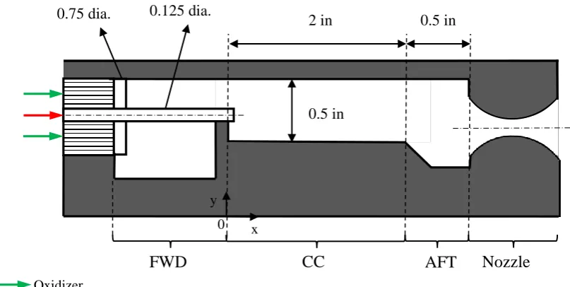
3. DESCRIPTION OF PHYSICAL MODEL
The Low Temperature Pressure Rocket Motor (LPRM) consists of oxygen plenum
(FWD), combustion chamber (CC), mixing chamber (AFT) and a nozzle as presented in
Figure 1.
Figure 1. Physical model of the LPRM
Fuel (methane) enters to the system through 0.125 inch – diameter tube while oxidizer
(oxygen) is supplied to the CC after straightened in FWD section. FWD section is not
modeled in detail in the present study for simplicity. Cross sections of fuel and oxidizer tubes
are first transformed to rectangular-shape by keeping inlet area same therefore flow variables,
i.e. velocity and mass flow rate do not change. Width of the LPRM is 1.5 in. so aspect ratio is
3. Then the cross section of LPRM on x-y plane is considered as 2-D physical model of
LPRM.
Reaction is initiated by ignition element at the outlet of fuel line. Assuming full
combustion of fuel, oxygen and products flow through CC and exit from nozzle.
FWD CC AFT Nozzle
0.5 in 2 in 0.125 dia.
0.75 dia.
Oxidizer Fuel
y
x 0
4
Following assumptions are made in order to develop the mathematical model:
1. The flow of oxygen and products are viscous, turbulent, subsonic, compressible and
steady-state.
2. LPRM walls are adiabatic with an emissivity of 1.
3. Turbulent flow is formulated based on a two equation standard k-ε model.
4. Radiative heat transfer is modeled by P-1 Radiation model.
In order to simulate the reacting flow, the geometry of the combustion chamber of the
LPRM is simplified. Several flow geometries are constructed to understand the characteristics
of flow and reaction. First, a channel model (Ch) is developed as presented in Figure 2.
Figure 2. Simplified geometry, Ch, for the present study
In geometry Ch, fuel is supplied at x = 0 and oxidizer feeds reaction. Reaction occurs
around x = 0 and oxidizer and products leave combustion chamber at x = L = 2 in. In this
simplified model, FWD is considered to be a 2-D, constant area channel and AFT and Nozzle
are not included in this configuration.
H = 0.5 in height of LPRM
hox,i= 2 x 0.125 in. height of oxidizer inlet
hf,i = 0.01 in height of fuel inlet
ho = 0.375 in height of outlet
L
H
x y
5
The other simplified model, CCNF, is the most comprehensive model consisting
FWD, CC, AFT and converging part of nozzle as presented in Figure 3.
Figure 3. Schematic of simplified model, CCNF
The real LPRM geometry allows oxidizer flow at x < 0. Because of the transformation
to two dimensional plane geometry, the fuel pipe acts as a restriction to oxidizer. Therefore, a
secondary oxidizer inlet is added in order to simulate the 3-D effects at the combustion
chamber inlet, although there is no secondary oxidizer inlet in the actual LPRM. X
Y
0 0.01 0.02 0.03 0.04 0.05 0.06 0.07
0 0.01 0.02
H = 0.5 in height of LPRM
hox,i= 2 x 0.125 in. height of oxidizer inlet
hf,i = 0.01 in height of fuel inlet
ho = 0.125 in height of outlet
LCC = 2 in Length of CC
LAFT = 0.5 in Legth of AFT
Secondary Oxidizer Fuel
Primary Oxidizer
Outlet
6
4. EXPERIMENTAL STUDY
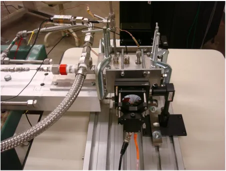
4.1.Description of the Experimental Setup
The experimental test setup consists of methane (CH4), gaseous oxygen (GO2) and
gaseous nitrogen (GN2) supply tanks, the test stand, a series of pipes, fittings and valves,
pressure gauges, pressure and differential pressure transducers, thermocouples, the LPRM
and Data Acquisition (DAQ) system. Test setup is presented in Figure 4 and Figure 5.
7
Figure 5. Low-Pressure Rocket Motor (LPRM)
Methane and oxygen are supplied from the pressurized supply tanks by regulating the
flow with control valves. Methane flows through the middle pipeline and temperatures and
pressures are measured by thermocouples and pressure transducers respectively and recorded
by DAQ system. Flow rates of methane and oxygen are adjusted using needle valves located
at the upstream of the LPRM.
LPRM consists of an oxygen plenum (FWD), combustion chamber (CC), a mixing
chamber (AFT) and a nozzle (N). Methane enters LPRM through CC and oxygen enters
FWD sections. Combustion takes place downstream of methane line in the CC, where
ignition is accomplished by electric igniter. Combustion products and oxidizer exits LPRM
8
LPRM is made of alumina silicate ceramic because of its high corrosion resistance
and low thermal expansion. Stainless steel sheets are used in order to secure mechanical
stability and reduce vibration. LPRM consists of one pressure transducer and four K-type
thermocouples (three for the flame and one for the chamber). In Figure 6, inside of LPRM
(top view) is presented indicating different sections of motor and thermocouples.
Figure 6. Inside view of LPRM and locations of thermocouples
Quarter inch quartz viewports are located at the both side of the LPRM to observe the
flame.
Piping and instrumentation diagram of the test setup is presented in Figure 7.
Instruments used in the experiments are listed in Appendix I. T/C 1
T/C 2
T/C 3 0.25"
FWD CC AFT Nozzle
9
Figure 7.Piping (and Instrumentation) diagram of the test setup
4.2.Experimental Procedure and Operating Conditions
Before starting the experiment, the pressure transducers at the methane inlet and
combustion chamber are calibrated. Calibration curves are presented in Appendix II.
Experimental procedure is listed below:
1. Thermocouples, pressure and differential pressure transducers and DAQ system are
checked and calibrated. LPRM is purged with gaseous nitrogen.
2. Methane tank pressure is set to the operating pressure value.
3. DAQ system is started.
4. Methane and oxygen are injected to LPRM by adjusting their flow rate values to
10
5. Methane is ignited by the electric igniter. If methane is not ignited, LPRM is purged
with nitrogen.
6. After a course of time (see operating conditions), needle valves are shut down and the
system is cooled down.
7. DAQ is stopped and the system is purged.
4.3.Data Analysis
Mass flow rate of methane is calculated using the change of pressure measured by the
differential pressure transducer. These calculations are based on Equations presented in
11
5. NUMERICAL STUDY
In this chapter, the mathematical model of the LPRM which is used in the numerical
simulations is presented. Governing differential equations and boundary conditions for the
proposed mathematical model are presented in Section 5.1 based on the assumptions listed in
Chapter 3. Solution technique is discussed in Section 5.2. ANSYS Fluent is used as a solver.
5.1.Mathematical Formulation
The governing differential equations for viscous, turbulent, compressible, unsteady
flow of a Newtonian fluid in 2–D planar Cartesian coordinates are presented below. Vector
form of the equations are presented in Appendix IV.
Continuity equation is given by:
0
( u ) ( v )
t x y
(1)
The momentum equation in the x- and y-direction become:
22 3 0 eff eff p u
( u ) uu uv V
t x y x x x
u v
y y x
(2) 2 2 0 3 eff eff
p v u
( v ) ( vu ) ( vv )
t x y y x x y
v V y y (3) respectively.
where µeff is the effective viscosity and defined as µeff = µ + µt and µt is the eddy viscosity
12 2 t k C (4)
where k and ε are turbulence kinetic energy and turbulence dissipation rate respectively and
Cµ is a constant. Transport equations for the Standard k – ε model are given as:
2 0 t t k k t k kk uk vk
t x y x Pr x y Pr y
S (5)
2 21 2 0
t t
t
u v
t x y x Pr x y Pr y
C S C
k k (6)
where Prk and Prε are turbulent Prandtl numbers for k and ε,Cε1 and Cε2 are constants
respectively. For this model, constants have the following values [19]:
Prk = 1.0, Prε = 1.3, Cε1 = 1.44 and Cε2 = 1.92
S is the modulus of the mean rate of strain tensor, which is defined as:
2 ij ij
S S S
The energy equation is given by:
0
p p p eff eff
r gen j
T T
c T c uT c vT k k
t x y x x y y
Q Q D
13
cp is the specific heat of the mixture which is found as: p i p ,i
i
c
Y c and specific heats ofindividual species are calculated using 4th order polynomials [20].
keff is the effective thermal conductivity and defined as: eff p t
t c k k Pr
Φ is the viscous dissipation term
r
Q is the radiative heat transfer which is found using P-1 Radiation model ([21], [22]) as:
2 4
4
r
Q aG anT (8)
where G is the incident radiation and can be found from the following equation:
1
4 2 4 03 a s Cs G aG an T
(9)
where a is the absorption coefficient, n is the refractive index of the medium and σ is
Stefan-Boltzmann constant.
gen
Q is the source of energy due to chemical reaction which is defined as:
j gen j j j H Q R M
(10)where Hj is the enthalpy of formation of species j and Rj is the rate of creation of species j.
Dj is equal to j j j
j
D
h J which represents the energy transfer due to species diffusionwhere Jj is the diffusion flux of species j which is defined for turbulent flows as:
t
i i ,m i T ,i
T
J D Y D
Sc T
14
where Dm,i and DT,i are mass and thermal diffusion coefficients respectively and Sc is the
Schmidt number which is defined as t t Sc D .
And transport of species is modeled as
1
0
t i m ,i T ,i
t i
m ,i T ,i i
( Y ) ( u Y ) ( vY ) Y T
i i i D D
t x y x Sc x T x
Y T
D D R
y Sc y y
(12)
where Yi is the mass fraction of ith species. Ri is the net rate of production of species i by
chemical reaction. There are several models to describe rate of production. In this study,
Laminar Finite Rate Model (LFRM) and Eddy-Dissipation Model (EDM) are compared and a
solution procedure is suggested which utilizes both reaction models.
LFRM computes the species source terms using Arrhenius chemical kinetics. The net
source of species i due to reaction is calculated as:
1
j
N p r
i i i i f j j
R M k C
(13)where
Mi is the molecular mass of species i
r i
and p i
are the stoichiometric coefficients for reactant and product respectively,
kf is the Arrhenius reaction rate and defined as:
r
E / RT f r
k A e where Ar is the pre-exponential factor, Er is the activation energy for the
15
Cjis the molar concentration of each reactant and product species j.
EDM calculates Ri by taking the minimum value of the following two expressions:
r R
i ,r i i R r
i ,R R
P
r P
i ,r i i N
p
j j
j
Y
R M A min
k M
Y
R M AB
k M
(14)where A and B are empirical constants and equal to 4.0 and 0.5 respectively.
Combustion of methane takes place according to single reaction four species assumption:
4 2 2 2 2 2
CH O CO H O
Then the production rate of fuel, methane becomes:
0 2. 1 3.
f f f f ox
R M k C C using LFRM. The reaction rate by EDM changes according to
Equation 14.
Boundary conditions for the GDE are provided to Fluent solver as follows: Mass flow
rate of fuel and oxidizer are given at inlets. Prescribed oxidizer mass flow rate is determined
to provide a stoichiometric value for oxidizer to fuel mass ratio. Additionally, temperatures
are prescribed at inlets. Mass fraction of methane at fuel inlet is defined as 1.0 and mass
fraction of oxygen at oxidizer inlet(s) are defined as 0.7 except for Bunsen burner
simulations. In Bunsen burner simulations, air (YO2 = 0.23) is taken as oxidizer. At outlet,
pressure is given as the boundary condition. LPRM walls are modeled as adiabatic. All the
16 5.2.Solution Technique
The governing equations are solved in 2-D planar space by pressure based solver
provided by ANSYS Fluent. Coupled scheme is used for pressure-velocity coupling and
spatial discretization is done based on second – order upwind scheme.
In order to simulate viscous, turbulent, compressible, unsteady reacting flow of a
Newtonian fluid, the following models by ANSYS Fluent are used: Energy, Turbulence –
Standard k-epsilon, Radiation – P1, Species – Species Transport.
False (Pseudo)-transient under-relaxation method is also used for more robust
solutions.
Summary of the solver and calculation settings and solution methods are presented in
Table 1.
Table 1. Solver settings, solution methods and calculation methods for the present study
Solver Settings
Pressure – based 2 – D Planar Steady Solution Methods
Scheme – Coupled
Gradient – Least Squares Cell Based Pressure – 2nd Order
Discretization – 2nd Order Upwind Pseudo – Transient
Calculation Settings
Residual Criteria: 10-15 for Non-Reacting 10-9 for Reacting
For the numerical simulations of steady-state reacting flows, modeling ignition is very
difficult because the nature of chemical reactions is unsteady. ANSYS Fluent provides
17
imposed conditions are utilized as the initial guess of the iterative calculations. Ignition is
simulated by imposing high temperature (~1750 K) on a specified region close to fuel inlet (x
= 0 – 0.15 in, y = 0.245 – 0.255 in) as the initial guess. Convergence is another problematic
aspect of the reacting flow simulations. For this purpose, a solution procedure is utilized
which requires an iterative reduction of the assumed value of the fuel inlet temperature by the
user.
1. Initialize the simulation for non-reacting cold flow of fuel and oxidizer. Run until
convergence is attained.
2. Once Step 1 is complete, update fuel inlet boundary condition: Tfi = 1500 K. Run
until solution converges.
3. Turn on Reaction – LFRM, patch 1750 K to fuel inlet. Run until solution converges.
4. Update boundary condition for fuel inlet: Tfi = 1200 K. Patch 1750 K to the same
region. Run until convergence is achieved.
5. Repeat Step 4 for Tfi = 900, 600, 300 K.
6. Once a converged solution is obtained at Step 5, turn reaction model to EDM without
18
6. RESULTS
In this chapter, results of the experiments and the computational simulations are
presented. Results include the experiment results, simulation of benchmark cases, grid
independence study as well as comparison of the experimental and computational study and
finally the results of the parametric study.
6.1.Results of the Experiments
In the present study, the operating conditions in Table 2 are used for hot test runs.
Table 2. Operating conditions for the experiments
Gas Supply Tank
Regulator Setting
Needle valve Ignition Setting
Needle valve Steady State Setting
Fuel Methane 40 psig 10° 10° 5°
Oxidizer Oxygen 40 psig 20° 20° 10°
Purge Nitrogen 40 psig 0° 0° 0°
Additionally, the experimental matrix is presented in Table 3.
Table 3. Experimental matrix
Chamber Pressure Chamber
Temperature
Flame Temperatures 1, 2,3
Mass Flow Rate of Fuel
M M M C
M: measured, C: empirically calculated
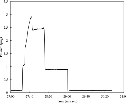
Two different runs are conducted with the same operating conditions. In this section,
results of the Run 1 are presented. Results of Run 2 are presented in Appendix VI. In Table 4,
results of Run 1 are tabulated and through Figure 8 to Figure 10, mass flow rate of methane,
chamber pressure, temperature of gases inside chamber and temperature of flame at the
19
Table 4. Chamber pressure, temperature, flame temperatures and mass flow rate of methane
Chamber Pressure
Chamber Temperature
Flame Temperature
Time T/C 1 T/C 2 T/C 3
Mass flow rate of fuel
(hh:mm:ss) [psig] [ᵒC] [ᵒC] [ᵒC] [ᵒC] [kg/s]
13:27:20 0.078 22.25 23.38 24.75 24.59 0
13:27:34 2.026 542.80 791.66 1090.40 1209.01 0.0001718
13:28:09 2.470 937.16 663.71 868.31 1066.80 0.0001487
13:28:51 0.886 478.33 713.26 1259.40 1364.75 0.0000701
13:29:05 0.074 285.41 592.18 635.59 578.80 0
20
Figure 8. Mass flow rate of methane versus time for Run 1
0 0.00005 0.0001 0.00015 0.0002 0.00025
27:00 27:40 28:20 29:00 29:40 30:20 31:00
Ma
ss
f
low
r
at
e
of
f
uel
(
k
g
/s)
Time (min:sec)
Ignition @ Valve
Setting 1 Valve Setting 2
21
Figure 9. Recorded chamber pressure (Pt) for Run 1
0 0.5 1 1.5 2 2.5 3 3.5
27:00 27:40 28:20 29:00 29:40 30:20 31:00
Pre
ss
ur
e
(psi
g
)
22
Figure 10. Registered temperatures (T/C) for Run 1
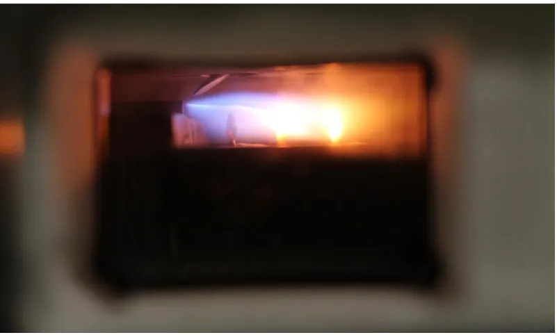
In addition to the experimental data presented above, pictures of the flame can be
found in Figure 11 and Figure 12.
0 200 400 600 800 1000 1200 1400 1600
27:00.0 27:40.0 28:20.0 29:00.0 29:40.0 30:20.0 31:00.0
T
em
per
at
ur
e
(°
C)
Time (min:sec)
Chamber Temperature Flame T/C 1
Flame T/C 2
Flame T/C 3
23
Figure 11. Picture of the flame from Run 1 at Valve Setting 1.
Figure 12. Picture of the flame from Run 1 at Valve Setting 2
6.2.Results of the Computational Model
In this section, results of the CFD simulations are presented. First, computational
model is validated using Benchmark case studies. Validation is done based on non-reacting
channel flow [23] and reacting flow in Bunsen burner. Additionally, simulations are verified
24
experimental results are compared and following that results of the parametric study are
introduced.
Operational parameters used in the computational studies are presented in Table 5.
Table 5. Operational Parameters in the simulations
Parameter Symbol Value Unit
Inlet mass flow rates
Fuel mf * kg/s
Oxidizer mox * kg/s
Inlet Mass Fraction
Fuel Yf,in 1.0 -
Oxidizer Yox,in * -
Inlet Temperature Tin 300 K
Outlet Pressure` Po * kPa
*Variable. See corresponding sections.
6.2.1. Validation of Computational Model
6.2.1.1. Flow Characteristics
In order to validate the computational model, the study of Morihara et al. [23] is
selected as a benchmark case. The authors presented the numerical solution to the flow in the
entrance region of a semi-infinite parallel channel for various Reynolds numbers. Solutions
for Re = 20, 200, and 2000 are considered as the benchmark case for the present study. A
semi-infinite plate with a 0.05 m height is modeled and results are nondimensionalized in
25
In Table 6, the results of the present study and results of the benchmark case are
tabulated. In Figure 13, these tabulated results are plotted.
Table 6. Non-dimensional centerline velocities of present study and Morihara et al.
Re 20 200 2000
x' B.C. P.S. % Dev. B.C. P.S. % Dev. B.C. P.S. % Dev.
0 1.00 1.00 0.00 1.00 1.00 0.00 1.00 1.00 0.00
0.005 1.01 1.006 -0.40 1.07 1.09 1.87 1.167 1.16 -0.60
0.01 1.03 1.022 -0.78 1.18 1.172 -0.68 1.23 1.233 0.24
0.015 1.05 1.048 -0.19 1.23 1.23 0.00 1.283 1.289 0.47
0.02 1.085 1.082 -0.28 1.28 1.276 -0.31 1.323 1.332 0.68
0.025 1.12 1.123 0.27 1.32 1.315 -0.38 1.361 1.367 0.44
0.03 1.18 1.165 -1.27 1.35 1.346 -0.30 1.389 1.394 0.36
0.035 1.22 1.208 -0.98 1.375 1.372 -0.22 1.414 1.415 0.07
0.04 1.26 1.249 -0.87 1.395 1.393 -0.14 1.431 1.431 0.00
0.06 1.37 1.376 0.44 1.45 1.447 -0.21 1.473 1.469 -0.27
0.08 1.44 1.443 0.21 1.47 1.471 0.07 1.485 1.484 -0.07
26
Figure 13. Comparison of non-dimensional centerline velocities predicted by the present study and by Morihara et al. for Re = 20,200, and 2000
6.2.1.2. Reacting Flow
Before carrying out the simulations of combustion inside LPRM model, flow in a
Bunsen burner in Ch geometry is simulated. Results are obtained for three different oxidizer
mass flow rates. Additionally, two different reaction models provided by ANSYS Fluent are
utilized.
In Table 7, operating conditions and general results for the Run Ch-R-I are presented.
1.0 1.1 1.2 1.3 1.4 1.5
0 0.02 0.04 0.06 0.08
N
ondi
m
ens
ional
v
el
oci
ty
,
u
Nondimensional distance, x
27
Table 7. Operating conditions and results for Run Ch-R-I
Run Number: Ch-R-I RESULTS
mf mo Po Pin mo Vo To
kg/s kg/s kPa kPa kg/s m/s K
0.0008 0.01 0 0.0018 0.01008 2.4 819
0.0008 0.02 0 0.0037 0.02008 3.4 624
0.0008 0.04 0 0.0085 0.04008 5.3 472
(a) (b) (c)
Figure 14. Temperature distribution (in Kelvins) for Bunsen burner inside Channel simulation with Eddy – Dissipation Reaction model for different mass flow rates of oxidizer: (a) mox=
0.01 kg/s, (b) mox= 0.02 kg/s, mox= 0.04 kg/s
Bunsen burner is also modeled with LFRM without employing Step 5 of the solution
procedure. As can be seen in Figure 15, LFRM over-estimates the flame temperature.
x (m)
y
(m
)
0 0.01 0.02
-0.01 0 0.01 0.02 0.03 0.04 0.05 0.06 x (m) y (m )
0 0.01 0.02
-0.01 0 0.01 0.02 0.03 0.04 0.05 0.06 x (m) y (m )
0 0.01 0.02
28
Therefore, for the other reacting flow simulations, all the steps of solution procedure, which
involve ED reaction model, are followed exactly.
Figure 15. Temperature distribution (in Kelvins) inside Channel for Bunsen Burner simulation with Laminar Finite Rate Reaction model
6.2.2. Grid Independence Study
Grid (mesh) independence study is conducted for non-reacting and reacting flows
separately. Only Channel (Ch) model is taken into consideration because the other geometries
are generated based on Channel.
Four different grids are constructed for this study. All of them are stretched in y –
direction and three of them are also stretched in x – direction. Stretching is geometric with a
growth rate 1.1. Characteristics of these grids are summarized in Table 8. These grids are
presented in Figure 16 and Figure 17.
x (m)
y
(m
)
0 0.01 0.02
29
Table 8. Properties of different meshes
Mesh Number of Cells along
x and y direction Stretching
1 105 x 72 Only y - direction
2 140 x 80 x and y direction
3 150 x 88 x and y direction
4 160 x 94 x and y direction
Figure 16. Mesh 1
Figure 17. Mesh 2, 3 and 4
x (m)
y
(m
)
-0.005 0 0.005
0 0.005 0.01 x (m) y (m )
0 0.02 0.04 0.06
0 0.005 0.01 0.015 0.02 x (m) y (m )
-0.005 0 0.005
0 0.005 0.01 x (m) y (m )
0 0.01 0.02 0.03 0.04 0.05 0.06 0.07
30 6.2.2.1. Non-Reacting Flow
In order to check that accuracy of the predictions and convergence of solutions are
independent of the selected grid size, simulations of non-reacting flows are considered. For
this purpose, mixing flow of methane and oxygen is simulated inside the Channel
configuration. Results are compared based on velocity and methane mass fraction profiles
along centerline and along a vertical line near the fuel inlet.
Table 9. Operating parameters and results for Run Ch-NR-I
Run Number: Ch-NR-I RESULTS
Mesh mf mo Po Pin mo Vo
kg/s kg/s kPa kPa kg/s m/s
Mesh 1 0.00066 0.01056 0 0 0.01122 1.02
Mesh 2 0.00066 0.01056 0 0 0.01122 1.04
Mesh 3 0.00066 0.01056 0 0 0.01122 1.08
Mesh 4 0.00066 0.01056 0 0 0.01122 1.07
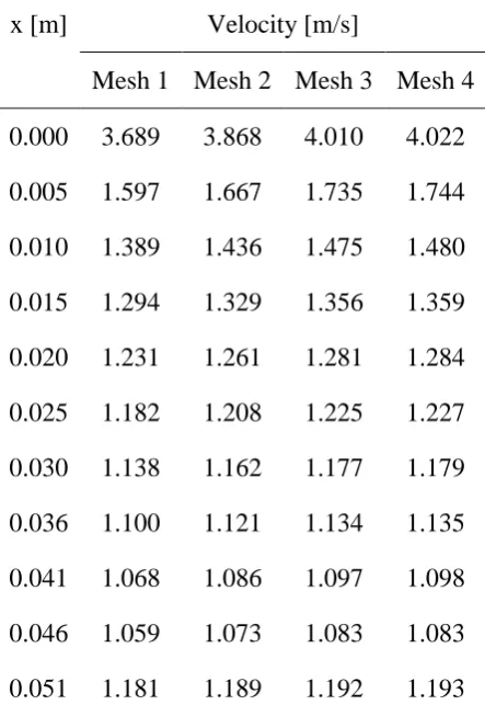
31
Table 10. Axial velocity along centerline using different meshes
x [m] Velocity [m/s]
Mesh 1 Mesh 2 Mesh 3 Mesh 4
0.000 3.689 3.868 4.010 4.022
0.005 1.597 1.667 1.735 1.744
0.010 1.389 1.436 1.475 1.480
0.015 1.294 1.329 1.356 1.359
0.020 1.231 1.261 1.281 1.284
0.025 1.182 1.208 1.225 1.227
0.030 1.138 1.162 1.177 1.179
0.036 1.100 1.121 1.134 1.135
0.041 1.068 1.086 1.097 1.098
0.046 1.059 1.073 1.083 1.083
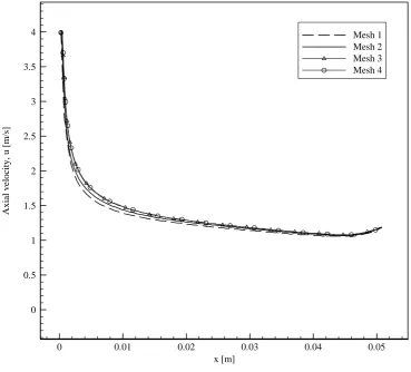
32
Figure 18. Axial velocity along centerline of Ch using different meshes
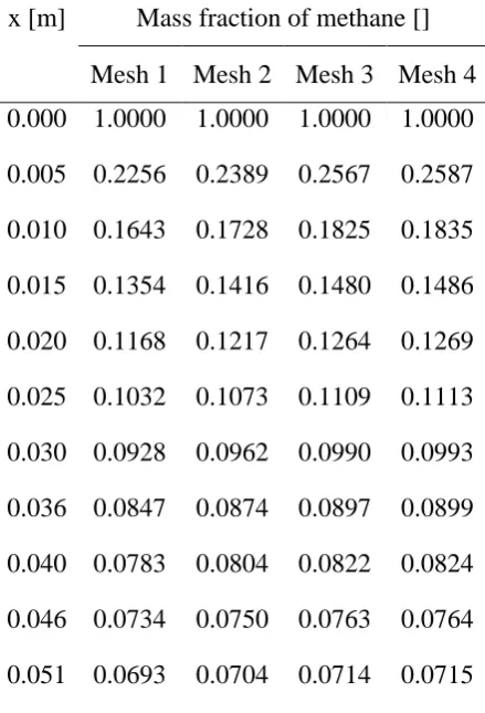
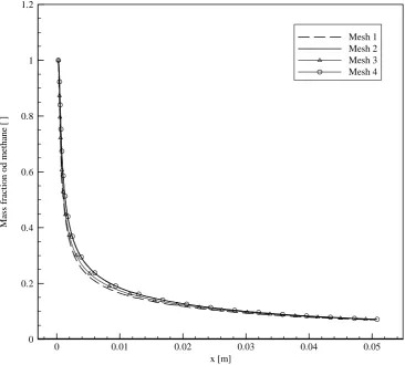
Mass fraction of methane along centerline is tabulated in Table 11 and plotted in
Figure 19.
x [m]
A
x
ia
l
v
el
o
ci
ty
,
u
[m
/s
]
0 0.01 0.02 0.03 0.04 0.05
0 0.5 1 1.5 2 2.5 3 3.5
4 Mesh 1
33
Table 11. Mass fraction of methane along centerline using different meshes
x [m] Mass fraction of methane []
Mesh 1 Mesh 2 Mesh 3 Mesh 4 0.000 1.0000 1.0000 1.0000 1.0000
0.005 0.2256 0.2389 0.2567 0.2587
0.010 0.1643 0.1728 0.1825 0.1835
0.015 0.1354 0.1416 0.1480 0.1486
0.020 0.1168 0.1217 0.1264 0.1269
0.025 0.1032 0.1073 0.1109 0.1113
0.030 0.0928 0.0962 0.0990 0.0993
0.036 0.0847 0.0874 0.0897 0.0899
0.040 0.0783 0.0804 0.0822 0.0824
0.046 0.0734 0.0750 0.0763 0.0764
34
Figure 19. Mass fraction of methane along centerline using different meshes
In addition to centerline, a vertical line near fuel inlet (x = 0.00127) is also taken into
account. Axial velocity distribution is tabulated in Table 12 and plotted in Figure 20.
x [m]
M
as
s
fr
ac
ti
o
n
o
d
m
et
h
an
e
[
]
0 0.01 0.02 0.03 0.04 0.05
0 0.2 0.4 0.6 0.8 1 1.2
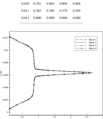
35
Table 12. Axial velocity along vertical axis at x = 0.00127 m
y [m] Axial velocity [m/s]
Mesh 1 Mesh 2 Mesh 3 Mesh 4 0.000 0.000 0.000 0.000 0.000
0.001 0.382 0.369 0.370 0.369
0.003 0.781 0.801 0.805 0.806
0.005 0.874 0.867 0.870 0.871
0.008 0.874 0.867 0.870 0.871
0.010 0.781 0.801 0.805 0.806
0.011 0.382 0.369 0.370 0.369
0.013 0.000 0.000 0.000 0.000
Figure 20. Axial velocity along vertical axis at x = 0.00127 m
Axial velocity, u [m/s]
y
[m
]
0.5 1 1.5 2 2.5 3
0 0.002 0.004 0.006 0.008 0.01 0.012
36
Axial velocity distribution along x = 0.00127 m is tabulated in Table 13 and plotted in
Figure 21.
Table 13. Mass fraction of methane along vertical axis at x = 0.00127 m
y [m] Mass fraction of methane [ ]
Mesh 1 Mesh 2 Mesh 3 Mesh 4 0.000 0.0000 0.0000 0.0000 0.0000
0.001 0.0000 0.0000 0.0000 0.0000
0.003 0.0000 0.0000 0.0000 0.0000
0.005 0.0017 0.0003 0.0002 0.0002
0.006 0.4492 0.4681 0.5159 0.5221
0.008 0.0017 0.0003 0.0002 0.0002
0.010 0.0000 0.0000 0.0000 0.0000
0.011 0.0000 0.0000 0.0000 0.0000
37
Figure 21. Mass fraction of methane along vertical axis at x = 0.00127 m
6.2.2.2. Reacting Flow
Similar to Non-reacting flow simulation, Ch-NR-I, different meshes are used to
simulate reacting flow inside the Channel geometry. Mesh 1 is eliminated for this run and
only the meshes which are stretched in both directions are used.
Mass fraction of methane [ ]
y
[m
]
0 0.1 0.2 0.3 0.4 0.5 0.6
0.004 0.005 0.006 0.007 0.008 0.009
38
Table 14. Operating conditions and results for Run Ch-R-II
Run Number: Ch-R-II RESULTS
Mesh mf mo Po Pin mo Vo To
kg/s kg/s kPa kPa kg/s m/s K
Mesh 2 0.0009 0.026 10 10.0 0.0269 11.3 1639
Mesh 3 0.0009 0.026 10 10.0 0.0269 11.7 1784
Mesh 4 0.0009 0.026 10 10.0 0.0269 11.6 1765
Comparison of these three grids are done based on the axial velocity and temperature
along centerline.
Axial velocity along centerline is tabulated in Table 15 and plotted in Figure 22.
Table 15. Axial velocity along centerline for Run Ch-R-II
x [m] Velocity [m/s]
Mesh 2 Mesh 3 Mesh 4
0.000 5.37 5.37 5.35
0.005 5.64 5.57 5.58
0.010 6.09 5.89 5.88
0.015 6.87 6.56 6.53
0.020 7.74 7.36 7.32
0.025 8.58 8.17 8.13
0.030 9.34 8.94 8.89
0.036 10.00 9.64 9.59
0.041 10.50 10.26 10.23
0.046 11.16 11.04 11.02
39
Figure 22. Axial velocity along centerline for Run Ch-R-II
Temperature along centerline is tabulated in Table 16 and plotted in Figure 23.
x [m]
A
x
ia
l
v
el
o
ci
ty
,
u
[m
/s
]
0 0.01 0.02 0.03 0.04 0.05
2 4 6 8 10 12 14 16
40
Table 16. Temperature along centerline for Run Ch-R-II
x [m] Temperature [K]
Mesh 2 Mesh 3 Mesh 4
0.000 328.0 308.1 306.2
0.005 1163.9 1049.3 1038.9
0.010 1514.7 1378.5 1364.7
0.015 1770.8 1620.8 1604.6
0.020 2001.3 1845.9 1827.4
0.025 2205.8 2068.8 2050.5
0.030 2362.9 2261.3 2246.7
0.036 2463.4 2400.8 2391.0
0.041 2448.8 2472.5 2471.7
0.046 2358.4 2417.8 2425.2
41
Figure 23. Temperature along centerline for different meshes
Based on the results presented in Sections 6.2.2.1 and 6.2.2.2, Mesh 3 is decided to be
used in the following simulations since there are minor differences in the results of Mesh 3
and the finer mesh, Mesh 4.
6.3.Comparison of Computational and Experimental Results
Computational model is calibrated based on experimental data by modifying specific
heats of combustion products, carbon dioxide and water vapor. Increasing specific heats
provided more reasonable temperature distribution in LPRM especially at high temperatures.
Specific heats of the products are taken as constant at two temperature bands differently. The
suggested specific heats are:
x [m]
T
em
p
er
at
u
re
,
T
[K
]
0 0.01 0.02 0.03 0.04 0.05
0 500 1000 1500 2000 2500 3000
42
cp,CO2= 1000 J/kg-K and cp,H2O= 1000 J/kg-K for 300 < T < 1000 K
cp,CO2= 2000 J/kg-K and cp,H2O= 5500 J/kg-K for 1000 < T < 5000 K
Although constant specific heat is not very reasonable approach for reacting flows, it
provides idea about modifying specific heats. The specific heats of all species must be
modified. Here, the results based on the proposed modified specific heats are presented.
Results of the computational simulations are compared to experimental data by temperature
taken from the specific locations in the experiments. Second phase of the Run 1 (2nd Valve
Setting) is selected for comparison. Operating conditions and the results for the
computational simulation is presented in Table 17. In Table 18, the comparison of
computational and experimental results is made and plotted in Figure 24. The experimental
values of temperature presented in this table are for time, to t = 13:28:51.
Table 17. Operating conditions and results for CCNF-R-I
Run Number: CCNF-R-I RESULTS
mf mo Po Pin mo Vo RR To
kg/s kg/s kPa kPa kg/s m/s kmol/ m3s K
0.0009 0.026 10 10.2 0.0269 35.7 26.1 1524
Table 18. Temperature values at thermocouple points
x [m] Temperature [K] % Difference
CFD Exp.
0.00635 1070.6 986.41 8.53
0.01270 1472.3 1532.55 -3.93
43
Figure 24. Temperature histogram at y = 0.15 along horizontal axis from Run CCNF-R-I compared with measured data from Run 1.
Through Figure 25 to Figure 31, temperature, pressure, density and mass fractions of
methane and products are presented for the Base case study.
Figure 25. Temperature distribution (in Kelvins) inside CCFN for Run CCNF-R-I
+ +
+
x [m]
T
em
p
er
at
u
re
[
K
]
0 0.02 0.04 0.06
0 500 1000 1500 2000 2500
CCNF-R-I Experiment
+
x (m)
y
(m
)
0 0.01 0.02 0.03 0.04 0.05 0.06 0.07
0 0.005 0.01 0.015 0.02
44
Figure 26.Pressure distribution (in Pascals) inside CCFN for Run CCNF-R-I
Figure 27. Predicted x-velocity (in m/s) inside CCFN for Run CCNF-R-I
Figure 28. Density (in kg/m3) variation inside CCFN for Run CCNF-R-I x (m)
y
(m
)
0 0.01 0.02 0.03 0.04 0.05 0.06 0.07
0 0.005 0.01 0.015 0.02
Pressure: 10010 10030 10050 10070 10090 10110 10130 10150 10170 10190
x (m)
y
(m
)
0 0.01 0.02 0.03 0.04 0.05 0.06 0.07
0 0.005 0.01 0.015 0.02
X Velocity: 0 2 4 6 8 10 12 14 16 18 20 22 24 26 28 30 32 34 36 38
x (m)
y
(m
)
0 0.01 0.02 0.03 0.04 0.05 0.06 0.07
0 0.005 0.01 0.015 0.02
Density: 0.2 0.3 0.4 0.5 0.6 0.7 0.8 0.9 1 1.1 1.2 1.3 [kPa]
[m/s]
45
Figure 29. Mass fraction of CH4 inside CCFN for Run CCNF-R-I
Figure 30. Mass fraction of CO2 inside CCFN for Run CCNF-R-I
Figure 31. Mass fraction of H2O inside CCFN for Run CCNF-R-I
As can be seen from Table 18 and Figure 24, computational results are in a good agreement
with experimental results. In this section, the computational model is verified that gives
0.05
0.1
0 0.60 0.30
x (m)
y
(m
)
0 0.01 0.02 0.03 0.04 0.05 0.06 0.07
0 0.005 0.01 0.015 0.02 0.05 0.05 0.05 0.10 0.10
0.15 0.15
0.15 0.20
0.20 0.25
0.25 0.30
0.30
x (m)
y
(m
)
0 0.01 0.02 0.03 0.04 0.05 0.06 0.07
0 0.005 0.01 0.015 0.02 0.05 0.05 0.10 0.10 0.10 0.15 0.15 0.15 0.20 0.20 0.25 0.27 x (m) y (m )
0 0.01 0.02 0.03 0.04 0.05 0.06 0.07
46
reasonable results. In the following sections of this thesis, effect of the several parameters are
investigated in order to provide data to the design of combustion experiments in the future.
Detailed list of the parameters used in Run CCFN-R-I can be found in Appendix VII.
6.4.Parametric Study
In this section, effects of several parameters are investigated on flow and combustion
characteristics in order to provide insight for the experiments to be conducted in the near
future. These parameters are mass flow rates of fuel and oxidizer and outlet pressure.
6.4.1. Effect of Different Mass Flow Rates
6.4.1.1. Effect of Fuel Mass Flow Rate
Operating conditions and results are presented in Table 19.
Table 19. Operating conditions and results for Run CCNF-R-II
Run Number: CCNF-R-II RESULTS
mf mo Po Pin mo Vo RR To
kg/s kg/s kPa kPa kg/s m/s kmol/ m3s K
0.0005 0.026 10 10.1 0.0265 25.6 26.1 1124
0.0009 0.026 10 10.2 0.0269 35.7 26.6 1524
0.0015 0.026 10 10.3 0.0275 46.9 28.6 1919
In Figure 32, temperature distributions inside CCNF are presented for various fuel
47 (a)
(b)
(c)
Figure 32. Temperature distribution (in Kelvins) inside CCNF for the Run CCNF-R-II. (a)
f
m = 0.0005 kg/s, (b) mf = 0.0009 kg/s, mf = 0.0015 kg/s
As the mass flow rate of fuel increases, high temperature region of the flow moves
through nozzle and mean temperature of the outflow increases. Although maximum x (m)
y
(m
)
0 0.01 0.02 0.03 0.04 0.05 0.06 0.07
0 0.005 0.01 0.015 0.02
Temperature: 300 400 500 600 700 800 900 1000 1100 1200 1300 1400 1500 1600 1700 1800 1900 2000 2100 2200 2300 2400 2500
x (m)
y
(m
)
0 0.01 0.02 0.03 0.04 0.05 0.06 0.07
0 0.005 0.01 0.015 0.02
x (m)
y
(m
)
0 0.01 0.02 0.03 0.04 0.05 0.06 0.07
0 0.005 0.01 0.015 0.02
48
temperature inside CCNF does not change significantly, high temperature region gets bigger
with the increasing fuel mass flow rate.
6.4.1.2. Effect of Oxidizer Mass Flow Rate
Operating conditions and results for Run CCNF-R-III are presented in Table 20.
Table 20. Operating conditions and results for Run CCNF-R-III
Run Number: CCNF-R-III RESULTS
mf mo Po Pin mo Vo RR To
kg/s kg/s kPa kPa kg/s m/s kmol/ m3s K
0.0009 0.013 10 10.1 0.0139 25.7 28.8 2071
0.0009 0.026 10 10.2 0.0269 35.7 26.6 1524
0.0009 0.050 10 10.5 0.0509 44.6 22.6 1025
In Figure 33, temperature distributions inside CCNF are presented for various
49 (a)
(b)
(c)
Figure 33.Temperature distribution (in Kelvins) inside CCNF for the Run CCNF-R-III. (a)
ox
m = 0.013 kg/s, (b) mox= 0.026 kg/s, mox= 0.05 kg/s
Oxygen acts as a cooling agent as well as an oxidizer for the fuel. Therefore, by
increasing oxidizer mass flow rate, chamber temperature can be decreased. x (m)
y
(m
)
0 0.01 0.02 0.03 0.04 0.05 0.06 0.07
0 0.005 0.01 0.015 0.02
Temperature: 300 400 500 600 700 800 900 1000 1100 1200 1300 1400 1500 1600 1700 1800 1900 2000 2100 2200 2300 2400 2500
x (m)
y
(m
)
0 0.01 0.02 0.03 0.04 0.05 0.06 0.07
0 0.005 0.01 0.015 0.02
x (m)
y
(m
)
0 0.01 0.02 0.03 0.04 0.05 0.06 0.07
0 0.005 0.01 0.015 0.02
50 6.4.2. Effect of Different Outlet Pressures
Operating conditions and results for Run CCNF-R-III are presented in Table 21.
Operating conditions and results for Run CCNF-R-I.
Table 21. Operating conditions and results for Run CCNF-R-IV
Run Number: RESULTS
mf mo Po Pin mo Vo RR To
kg/s kg/s kPa kPa kg/s m/s kmol/ m3s K
0.0009 0.026 10 10.2 0.0269 35.7 26.6 1524
0.0009 0.026 100 100.1 0.0269 19.8 30.6 1525
0.0009 0.026 300 300.1 0.0269 9.9 32.7 1525
In Figure 34, temperature distributions inside CCNF are presented for various fuel
51 (a)
(b)
(c)
Figure 34.Temperature distribution (in Kelvins) inside CCNF for the Run CCNF-R-IV. (a) Po = 10 kPa, (b) Po = 100 kPa, (c) Po = 300 kPa
As higher pressures are prescribed at outlet, pressure and density in the chamber
increases. Therefore, pressure has an indirect effect of the characteristics of combustion.
Higher reaction rates are attained with higher densities. Although maximum temperature does
not change significantly, temperature gradient of gases inside chamber decreases. x (m)
y
(m
)
0 0.01 0.02 0.03 0.04 0.05 0.06 0.07
0 0.005 0.01 0.015 0.02
Temperature: 400 500 600 700 800 900 1000 1100 1200 1300 1400 1500 1600 1700 1800 1900 2000 2100 2200 2300 2400
x (m)
y
(m
)
0 0.01 0.02 0.03 0.04 0.05 0.06 0.07
0 0.005 0.01 0.015 0.02
x (m)
y
(m
)
0 0.01 0.02 0.03 0.04 0.05 0.06 0.07
0 0.005 0.01 0.015 0.02
52
7. CONCLUSIONS
In this thesis, the reacting flow inside the LPRM is studied experimentally and
computationally. Experiments are conducted in University of New Orleans Combustion
Laboratory. Computational simulation has been done using ANSYS Fluent as a solver. Flow
inside the combustion chamber is modeled as viscous, turbulent and compressible in 2-D
planar domain. Mathematical modeling is done based on unsteady assumption. In CFD
simulations, pseudo – transient approach is utilized to determine steady – state temperature
distribution. Benchmark cases for non-reacting and reacting flows are considered to verify
the accuracy of the computational model. Four different mesh sizes are used for
determination of the most proper grid considering the accuracy of solutions and computation
time.
The following conclusions were drawn from the results of the simulations:
1. Benchmark case of flow between semi-infinite plates is taken and compared with the
results found in the present study. Results shows that the present mathematical model
gives accurate results for the Benchmark case considered.
2. A special solution procedure is constructed for the numerical simulations, which
utilizes different reaction models. Results show that this procedure provides an
accurate prediction for the location of chemical reaction as well as a reasonable
temperature distribution of gases inside LPRM.
3. The computational model is calibrated in order to obtain a reasonable gas temperature
distribution inside LPRM by modifying specific heats of products. After calibration,
there is a good agreement between the results obtained from computational model and
53
4. The results of the parametric study give idea about the effects of mass flow rates of
fuel and oxidizer and pressure at outlet to design the future experiments for non –
54
8. RECOMMENDATIONS
This thesis aimed to understand the characteristics of reacting flow of methane and
oxygen inside a low – pressure rocket motor. To improve the present study:
i. The base case CFD simulation is calibrated based on experimental results for
temperature by modifying specific heats of combustion products, i.e. carbon
dioxide and water vapor. Modification of specific heats should be according to the
data in the literature.
ii. CFD simulations should be repeated for unsteady reacting flow of methane and
55
REFERENCES
[1] E. Seedhouse, SpaceX: making commercial spaceflight a reality. Springer Science & Business Media, 2013.
[2] E. Seedhouse, Red Dragons, Ice Dragons, and the Mars Colonial Transporter. Springer International Publishing, 2016.
[3] K. M. Akyuzlu, H. Sayed, and Y. Pavri, “Determination of Regression Rate in Ablating Solid Fuels for Hybrid Rocket Motors Using a 2-D Subscale Low Pressure Test Bed,” in Ankara International Aerospace Conference, 2005.
[4] P. Dagaut, J.-C. Boettner, and M. Cathonnet, “Methane Oxidation: Experimental and Kinetic Modeling Study,” Combust. Sci. Technol., vol. 77, no. 1–3, pp. 127–148, 1991.
[5] G. B. Skinner, A. Lifshitz, K. Scheller, and A. Burcat, “Kinetics of Methane Oxidation,” J. Chem. Phys., vol. 56, no. 8, pp. 3853–3861, 1972.
[6] F. N. Egolfopoulos, P. Cho, and C. K. Law, “Laminar flame speeds of methane-air mixtures under reduced and elevated pressures,” Combust. Flame, vol. 76, no. 3–4, pp. 375–391, 1989.
[7] T. C. Wagner and C. R. Ferguson, “Bunsen flame hydrodynamics,” Combust. Flame, vol. 59, no. 3, pp. 267–272, 1985.
[8] K. K. Kuo, Principles of Combustion. 1986.
[9] G. E. Andrews and D. Bradley, “The burning velocity of methane-air mixtures,” Combust. Flame, pp. 275–288, 1972.
[10] D. D. S. Liu and R. MacFarlane, “Laminar burning velocities of hydrogen-air and hydrogen-air steam flames,” Combust. Flame, vol. 49, no. 1–3, pp. 59–71, 1983.
[11] Y. C. Chen, N. Peters, G. a Schneemann, U. Wruck N. und Renz, and M. S. Mansour, “The Detailed Flame Structure of Highly Stretched Turbulent Premixed Methane-Air-Flames,” Combust. Flame, vol. 107, pp. 223–244, 1996.
[12] H. Kobayashi, K. Seyama, H. Hagiwara, and Y. Ogami, “Burning velocity correlation of methane/air turbulent premixed flames at high pressure and high temperature,” Proc. Combust. Inst., vol. 30, no. 1, pp. 827–834, 2005.
[13] S. Pfadler, M. L??ffler, F. Dinkelacker, and A. Leipertz, “Measurement of the conditioned turbulence and temperature field of a premixed Bunsen burner by planar laser Rayleigh scattering and stereo particle image velocimetry,” Exp. Fluids, vol. 39, no. 2, pp. 375–384, 2005.
56
[15] K. M. Akyuzlu, “Modeling of Instabilities Due to Coupling of Acoustic and
Hydrodynamic Oscillations in Hybrid Rocket Motors,” 43rd AIAA/ASME/SAE/ASEE Jt. Propuls. Conf. Exhib., no. July, pp. 1–11, 2007.
[16] K. M. Akyuzlu and K. Albayrak, “IMECE2011-64327 Thermal and Hydrodynamic Oscillations,” pp. 1–9, 2011.
[17] K. M. Akyuzlu, K. Albayrak, and C. Karaeren, “A Numerical Study of
Thermoacoustic Oscillations in a rectangular Channel Using CMSIP Method,” in ASME 2009 International Mechanical Engineering Congress and Exposition, 2009.
[18] A. Antoniou and K. Akyuzlu, “A physics based comprehensive mathematical model to predict motor performance in hybrid rocket propulsion systems,” 41st
AIAA/ASME/SAE/ASEE Jt. Propuls. Conf. Exhib. 10 - 13 July 2005, Tucson, Arizona, no. July, pp. 1–16, 2005.
[19] B. E. Launder and D. B. Spalding, Lectures in Mathematical Models of Turbulence. London: Academic Press, 1972.
[20] J. W. Rose, Technical Data on Fuels, 7th ed. Wiley, 1977.
[21] P. Cheng, “Two-Dimensional Radiating Gas Flow by a Moment Method,” AIAA J., vol. 2, pp. 1662–1664, 1964.
[22] R. Siegel and J. R. Howell, Thermal Radiation Heat Transfer. Washington D.C.: Hemisphere Publishing Corporation, 1992.
[23] H. Morihara and R. Ta-Shun Cheng, “Numerical solution of the viscous flow in the entrance region of parallel plates,” J. Comput. Phys., vol. 11, no. 4, pp. 550–572, 1973.
[24] Fluent, ANSYS FLUENT User ’ s Guide, vol. 15317, no. November. 2011.
57 APPENDIX – I
EQUIPMENT LIST USED IN THE EXPERIMENTS
Table I.1. LPRM Test Stand Equipment List
58
APPENDIX – II
CALIBRATION CURVES FOR THE EXPERIMENTS
MD2 CH0 Differential Pressure Transducer
Table II.1: Differential Pressure Transduer values taken to make a calibration curve.
Valve (rad)
Pressure Upstream
(psig)
Pressure Downstream
(psig)
Voltage (mV)
Delta P (psig)
0 40 40 0.01 0
π 40 40 0.03 0
2π 40 39.6 0.07 0.4
3π 40 39.1 0.12 0.9
4π 40 39.1 0.19 0.9
5π 40 38.6 0.28 1.4
6π 40 38.1 0.37 1.9
7π 40 38.1 0.49 1.9
8π 40 37.6 0.62 2.4
9π 39.9 37.1 0.76 2.8
10π 39.9 36.6 0.9 3.3
11π 39.9 36.1 1.05 3.8