Simultaneous Structure Coupled Joint Inversion of Gravity and Magnetic Data Based on a Damped Least Squares Technique

http://dx.doi.org/10.4236/ijg.2015.62011

How to cite this paper: Zhou, J.J., Xiu, C.X. and Zhang, X.D. (2015) Simultaneous Structure-Coupled Joint Inversion of Gravi-ty and Magnetic Data Based on a Damped Least-Squares Technique. International Journal of Geosciences, 6, 172-179. http://dx.doi.org/10.4236/ijg.2015.62011

Simultaneous Structure-Coupled Joint

Inversion of Gravity and Magnetic Data

Based on a Damped Least-Squares

Technique

Junjie Zhou1,2*_{, Chunxiao Xiu}1,2_{, Xingdong Zhang}1,2

1_{Key Laboratory of Geo-Detection (China University of Geosciences, Beijing), Ministry of Education, Beijing, China} 2_{School of Geophysics and Information Technology, China University of Geosciences, Beijing, China}

Email: *_{[email protected]}

Received 15 January 2015; accepted 12 February 2015; published 16 February 2015 Copyright © 2015 by authors and Scientific Research Publishing Inc.

This work is licensed under the Creative Commons Attribution International License (CC BY).

http://creativecommons.org/licenses/by/4.0/

Abstract

The structure-coupled joint inversion method of gravity and magnetic data is a powerful tool for developing improved physical property models with high resolution and compatible features; how-ever, the conventional procedure is inefficient due to the truncated singular values decomposition (SVD) process at each iteration. To improve the algorithm, a technique using damped least squares is adopted to calculate the structural term of model updates, instead of the truncated SVD. This pro-duces structural coupled density and magnetization images with high efficiency. A so-called coupling factor is introduced to regulate the tuning of the desired final structural similarity level. Synthetic examples show that the joint inversion results are internally consistent and achieve higher resolu-tion than separated. The acceptable runtime performance of the damped least squares technique used in joint inversion indicates that it is more suitable for practical use than the truncated SVD method.

Keywords

Structure-Coupled Joint Inversion, Damped Least-Squares, Coupling Factor, Gravity and Magnetic Data

1. Introduction

However, handling the combination of geophysical data types, each of which is sensitive to different material properties, poses a major challenge. In the early stage, Menichetti and Guillen [1] proposed a generalized in-verse method to recover 2.5-D models with fixed densities and susceptibilities. Serpa and Cook [2] inverted the densities, susceptibilities and the vertices of 2.5-D models with a priori information added. In recent years, some advanced numerical solutions were developed. Zeyen and Pous [3] were the first to study 3-D joint insion of magnetic and gravity data, presenting a quasi-Newton algorithm for a designed model composed of ver-tical rectangular prisms with fixed lateral boundaries parallel to the local coordinate system. Gallardo-Delgado et al. [4] proposed a versatile algorithm for joint 3-D inversion of gravity and magnetic data, with the depths to the tops and bottoms as unknowns to be determined. Pilkington [5] jointly processed the gravity and magnetic data in terms of a model consisting of an interface separating two layers with constant density contrast and magne-tization. Gallardo et al. [6] described and applied an automated refinement technique for 3-D multilayer models conditioned by gravity and magnetic data and by meaningful geometrical and physical constraints. The objective function they had used was a quadratic program in a stable iterative scheme, which produced models that corre-lated with the surface geology and revealed the subsurface features. Besides the layered model, a model includ-ing a large set of combined prisms is also preferred to approximately simulate the spatial variations of the phys-ical properties. Fregoso and Gallardo [7] presented a cross-gradients joint framework applicable to gravity and magnetic data. The kernel technique and structural similarity criterion were first applied to electrical and seismic data [8], and were then soon developed for other types of data [9] [10]. Zhdanov et al. [11] developed Gramian constraints for gravity and magnetic data to illustrate the effectiveness of the approach. Shamsipour et al. [12] presented a novel stochastic joint inversion method for gravity and magnetic data based on cokriging. To sum up, various methodologies of joint inversion for simultaneously handling these two kinds of data have been investi-gated, which is an indication of its importance and broad potential application.

In this study we present a joint inversion framework for gravity and magnetic data using a structural similarity criterion, which is proposed as an improved version of the Fregoso and Gallardo [7] approach when taking its practical application into consideration. First, the structural similarity criterion is reviewed in detail. Second, a cost function with cross-gradients component constraints is given, and iterative formula is presented based on the general nonlinear least-squares technique. The key issue in solving this problem concerns the structural vector updates at each iteration. Instead of conventional truncated singular value decomposition (SVD) adopted in pre-vious work, we propose a damped least-squares algorithm to carry out controlled structure resemblance and ef-ficient computation. We then test the method with several synthetic examples and compare the results obtained using mono-inversion of each dataset, and joint inversion of the integrated dataset, to demonstrate the reliability and efficiency of the proposed algorithm.

2. Joint Inversion Methodology

The principle of the structural similarity criterion is that collocated multiple physical property models that reflect the same geological structure are considered implicitly to have common boundaries. Therefore the structural si-milarity criterion is required to quantitatively evaluate the structural resemblance of one or two physical proper-ty models. Haber and Oldenburg [13] introduced a structural operator for conducting constraint inversion pro- cesses. Gallardo and Meju [8] extended the formula to the cross-product of two given model gradients, termed the “cross gradient”:

(

)

(

)

(

)

τ = ∇ ×∇ . (1)

where m1 and m2 are the two participating physical property values at an arbitrary subsurface location in 3-D space, and ∇ is the gradient operator. The model is a naturally continuous variable of x-, y- and z-geometrical measures; however, it is discretized with an aggregated prism set, which is suitable for carrying out numerical computations. The cross-gradients vector, τ , indicates the structural similarity at the current point. The vector can obviously be written as three orthometric components:

1 2 1 2_; 1 2 1 2_; 1 2 1 2_.

x m m_{y z} m m_{z y} y m m_{z x} m m_{x z} z m m_{x y} m m_{y x}

τ =∂ ∂ −∂ ∂ τ =∂ ∂ −∂ ∂ τ =∂ ∂ −∂ ∂

which express the structural similarity of the two models on their orthometric vertical projection surfaces. When the model gradients have the same or reverse direction, that is, their gradients are parallel, these three compo-nents tend to have very small values; otherwise they would be non-zero quantities. So, for the whole model vo- lume beneath the study area, a built-up array T_{, ,}T T T

x y z

 

=  

τ τ τ τ is used to measure the structural similarity

throughout the whole space. When the structures are consistent, the array τ should approach a null space 0. This property is what we have used as a structural constraint in the cost function in order to obtain the desired results with a good structural resemblance feature.

2.2. Cost Function of Joint Inversion

As described by Gallardo and Meju [8], joint inversion promises to reduce the set of solutions by combining var-ious data in a single scheme, and driving the updated model to explain all the requirements included in the cost function, such as data fitting, model smoothness, the distance of the model from prior information, and the struc-tural similarity. Thus the cost function is expressed as:

( )

( )

(

(

)

)

2

2 2

1 1 1 1 1 1 10

2 2 2 2 2 2 20

ˆ

min _ˆ , subject to

L

d C p

C C g g ϕ − − − − − = + + =

− − 0

p d Lp Z p p

p d Lp Z p p τ . (3)

where subscripts 1 and 2 represent the gravity and magnetic methods; subscript 0 represents reference vector in-formation; d is the observational data vector; p is the transformed model vector; gˆ is the transformed for-ward-modeling operator; the transform function between p and m is defined by the user to satisfy some known physical information; Z is the depth-weighting matrix [14]; L is the Laplacian matrix; C is the covariance matrix with respect to subscripts d (data), L(smoothness) and p (smallness), which are terms in the cost function; and τ

is the assembled cross-gradients three-component array. The cost function satisfies the equality constraint, which is mainly where it differs from unconstrained optimization frameworks. The structural constraints provide the correlation between model parameters that formulate the complete algorithm. When the two models are coupled in structure, the operator tends to reach null space 0.

Following the robust statistical optimization algorithm framework developed by Fregoso and Gallardo [7], the nonlinear generalized inversion problem that minimizes this cost function is solved so that the data and discrete model can be submitted into a general framework and can be processed simultaneously:

(

)

1 1 T 1 T 1

k k k k k k k k k k k k

−

− − − _ − _

∆ =p N n +N B B N B _B N n −τ _. (4)

where T T T

1, 2

 

=  

p p p is the combined model vector; N and n are a matrix and an array which involve the ma-trices described above; B is the cross-gradients Jacobian matrix with respect to m1 and m2; and k is the itera-tion number. The intermediate variables are expressed by:

( )

(

)

T 1 T 1 T 1

T 1 T 1 1

0

;

ˆ .

k d L p

k d g k L k p k

− − −

− − −

= + +

 

= _ − _+ + −

N J C J L C L Z C Z

n J C p d L C Lp C Z p p . (5)

where J is the combined and transformed forward modeling Jacobian matrix. The inverse of N may be calcu-lated by any conventional algorithm, and the inverse of _ −1 T_

BN B , which does not have to be computed

direct-ly, is presented in detail below. The model update in the kth iteration is then obtained by:

1

k+ = k + ∆ k

p p p . (6) The final models m1 and m2 are extracted from p by an inverse transform function when the iteration pro-cedure satisfies the given threshold concerned with data misfit and structural similarity.

2.3. Damped Least-Squares Technique The inverse of matrix _ −1 T_

BN B  is usually difficult to compute because the production of the several

(

)

k k k

+

− _{= Λ}−

B N B V U . (7)

where U and V are orthonormal matrices, and Λ is the corresponding singular value matrix. Then the recons-titution is expressed as:

(

)

k k k c c c

+

− _{= Λ}−

B N B V U . (8)

where c is the truncated index of the non-null singular sequence λ1≥λ2≥≥λc. However, this technique is not suitable for large-scale computations. Especially in the present case, the vectors are ready to compute in a combined manner, which enlarges the dimensions of both the model and the data. We suggest the use of an al-ternative algorithm to handle this problem. A damping factor is introduced to help improve the ill-posed feature of the matrix. The equation becomes:

(

)

1 T max k k k 1

k k k _β k k k k k

−

− −

 

 +  = −

 

 

B N B

B N B I t B N n τ . (9)

where I is the identity matrix, and β is the denominator of the damping factor. The second term added in brack-ets has the effect of making the total matrix well-posed. Although some structural perturbation information is lost in such a scheme, the computation stability is enhanced. This linear system is easy to compute with an itera-tive conjugate gradient solver, which accelerates the computing rates compared to truncated SVD. Then model updates of the equation at the kth iteration is solved using:

1 1 T

k k− k k− k k

∆ =p N n +N B t . (10)

which is the equation adopted in this paper. In this scheme, β is termed a coupling factor, and has an impact on the final achieved structural resemblance such that large values of β indicate greater model similarity. In other words, the structural coupling level may be readily controlled by tuning β by trial and error. A synthetic test be-low outlines the principle of choosing an optimal value of β.

3. Synthetic Examples

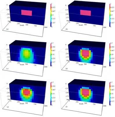
We first describe a synthetic example that illustrates the basic features of the proposed joint technique, using a typical synthetic model similar to that of Frogoso and Gallardo [7]. The subsurface was divided into a mesh of 20 × 20 × 10 rectangular elements with a 50 m space in the x-, y- and z-directions. The geological target was located at a roof depth of 100 m beneath the center of the study area. The density contrast was 1.0 g/cm3 _and magnetiza-tion amplitude was 1.0 A/m. Figure 1 shows the theoretically modeled gravity and total magnetic intensity ano-maly contaminated by 2.5% Gaussian noise, and the geomagnetic field was set as declination D = −5˚ and incli-nation I = 50˚. The separate inversion experiment was carried out by omitting the second term on the right-hand side of Equation (10), and the joint inversion was completed with _{β =5.0 10×} 4_{; the selection of this value is} ex-plained below. For gravity and magnetic inversions, the depth-weighting technique should be included to counte-ract anomaly concentrations near the surface. The reference models for both density and magnetization model are set to 0. The maximum number of iterations was 6.

Figure 2 shows the inversion results for both the separate and joint inversion cases. For reasons of symmetry, only the vertical profile on northing = 500 m is presented. All the results reflect the true geological target in a fuzzy manner. Considered separately, better recovery was obtained from the magnetization model than from the density model due to the greater sensitivity of the magnetic method; however, the density values were lower, and these results were distorted with a broad tail at depth. In the joint inversion, both the density model and magneti-zation model improved, with more focused features than when separate. A significant characteristic was that the resultant density and magnetization structure were consistent. Not only did the resultant compatible images en-hance the resolution, they also reduced the inherent non-uniqueness of the inverse problems. It is clear that the joint inversion technique incorporating the structural similarity constraint produced improved images with higher resolution.

0 N or thi ng ( m )

167 333 500 667 833 1000

Easting (m) 0 167 333 500 667 833 1000 0 N or thi ng ( m )

167 333 500 667 833 1000

Easting (m) 0 167 333 500 667 833 1000

nT −56.98

−26.55 3.886 34.32 64.75 95.19 125.6 0.009556 mGal 0.2399 0.4703 0.7006 0.931 1.161 1.392 Observed Gravity Data

400 data Observed Magnetic Data 400 data, I = 50, D = −5

Figure 1.Schematic of synthetic gravity data (a) and magnetic data (b). The black boxes indicate projected view of geological targets with different physical property feature.

South 250 ₅₀₀

750 1000 -375 -250 -125 0

(a) (b)

(d) (c)

(e) (f)

0 500

South 250

500 ₇₅₀

1000 -375 -250 -125 0 0 500 South 250 ₅₀₀

750 1000 -375 -250 -125 0 0 500 South 250 ₅₀₀

750 1000 -375 -250 -125 0 0 500 South 250 ₅₀₀

750 1000 -375 -250 -125 0 0 500 South

250 ₅₀₀ 750 1000 -375 -250 -125 0 0 500 0 0.167 0.333 0.5 0.667 0.833 1 0 0.167 0.333 0.5 0.667 0.833 1 0 0.117 0.233 0.35 0.467 0.583 0.7 0 0.117 0.233 0.35 0.467 0.583 0.7 0 0.117 0.233 0.35 0.467 0.583 0.7 0 0.117 0.233 0.35 0.467 0.583 0.7

1 2 3 4 5 6 # of iteration

10−7 10−6 10−5 10−4

β = 0.5

β = 5

β = 50

β = 500

β = 5000

β = 50,000

cr

os

s gr

adi

ent

s nor

m

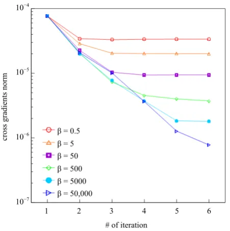
Figure 3.Cross-gradients norm convergence curves using dif-ferent structural coupling factor β.

structures are consistent with each other, while a large value accounts for the incompatible feature. Clearly, a large β value achieved better convergence than a small value; however, if too big, the stability of the computa-tion may be compromised. The choice often entails a trial-and-error process. A relatively large number may be chosen provided it achieves satisfactory convergence of the cross-gradients norm and that the numerical compu-tation is stable.

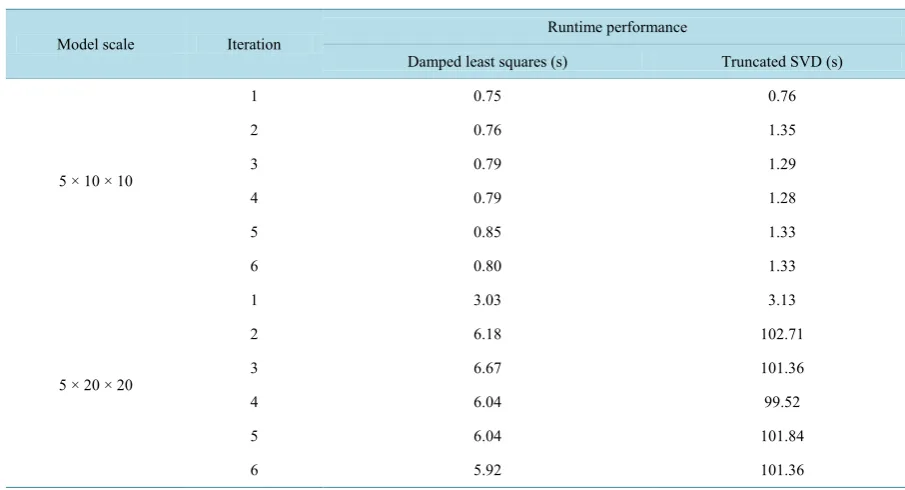
We then tested and compared the efficiency of the proposed damped least-squares technique and the conven-tional truncated SVD. Two different mesh discretization scales were adopted with various model dimensions to demonstrate runtime performance on the same computer platform. Table 1 shows that, for the smaller model scale, the damped method (final cross-gradients norm 8.3 × 10−8_{) was slightly faster than SVD (final cross-gradients} norm 3.9 × 10−8_{), but for the larger model scale, the runtime of the truncated SVD (final cross-gradients norm} 6.0 × 10−8_{) dramatically increased at each iteration except the initial computation, compared to the damped} me-thod (final cross-gradients norm 2.4 × 10−8_{). It was seen that the truncated SVD is not suitable for large-scale} problems. The damped least-squares method obtains the same results but with better runtime performance.

4. Conclusions

Efficient, simultaneous 3-D structure-coupled joint inversion of collocated gravity and magnetic data using a damped least-squares technique is presented. It is consistent with the previous view that the cross-gradients con-straints have a significant capacity to obtain more compatible models with higher structural resemblance than separated inversion.

The damped least-squares technique is introduced to perform efficient computation of the structural perturba-tion term in the linear system at each iteraperturba-tion. A coupling factor is proposed to regulate the final structural si-milarity level achieved. A relatively large value of this factor, chosen by trial and error, is suggested to achieve desired cross-gradients norm convergence on condition that the numerical computation is stable.

The synthetic experiments show that the joint inverted density and magnetization results are consistent, which reveals the geological setting. Furthermore, the runtime performance is more acceptable than that of truncated SVD, indicating its suitability for practical use.

Acknowledgements

Table 1.Runtime comparison of damped least squares and truncated SVD.

Model scale Iteration Runtime performance

Damped least squares (s) Truncated SVD (s)

5 × 10 × 10

1 0.75 0.76

2 0.76 1.35

3 0.79 1.29

4 0.79 1.28

5 0.85 1.33

6 0.80 1.33

5 × 20 × 20

1 3.03 3.13

2 6.18 102.71

3 6.67 101.36

4 6.04 99.52

5 6.04 101.84

6 5.92 101.36

Program) of China (No. 2013AA063901-4 and 2013AA063905-4), R&D of Key Instruments and Technologies for Deep Resources Prospecting (The National R&D Projects for Key Scientific Instruments) (No. ZDYZ2012- 1-02-04), Constrained multi-parameter inversion of geophysical technology and software systems (No. 2014AA06A613), and The Fundamental Research Funds for the Central Universities.

References

[1] Menichetti, V. and Guillen, A. (1983) Simultaneous Interactive Magnetic and Gravity Inversion. Geophysical

Pros-pecting, 31, 929-944. http://dx.doi.org/10.1111/j.1365-2478.1983.tb01098.x

[2] Serpa, L.F. and Cook, K.L. (1984) Simultaneous Inversion Modeling of Gravity and Aeromagnetic Data Applied to a Geothermal Study in Utah. Geophysics, 49, 1327-1337. http://dx.doi.org/10.1190/1.1441759

[3] Zeyen, H. and Pous, J. (1993) 3-D Joint Inversion of Magnetic and Gravimetric Data with a Priori Information.

Geo-physicalJournalInternational, 112, 244-256. http://dx.doi.org/10.1111/j.1365-246X.1993.tb01452.x

[4] Gallardo-Delgado, L., Pérez-Flores, M. and Gómez-Treviño, E. (2003) A Versatile Algorithm for Joint 3D Inversion of gravity and Magnetic data. Geophysics, 68, 949-959. http://dx.doi.org/10.1190/1.1581067

[5] Pilkington, M. (2006) Joint Inversion of Gravity and Magnetic Data for Two-Layer Models. Geophysics, 71, L35-L42. http://dx.doi.org/10.1190/1.2194514

[6] Gallardo, L.A., Pérez-Flores, M.A. and Gómez-Treviño, E. (2005) Refinement of Three-Dimensional Multilayer Mod-els of Basins and Crustal Environments by Inversion of Gravity and Magnetic Data. Tectonophysics, 397, 37-54. http://dx.doi.org/10.1016/j.tecto.2004.10.010

[7] Fregoso, E. and Gallardo, L.A. (2009) Cross-Gradients Joint 3D Inversion with Applications to Gravity and Magnetic data. Geophysics, 74, L31-L42. http://dx.doi.org/10.1190/1.3119263

[8] Gallardo, L.A. and Meju, M.A. (2004) Joint Two-Dimensional DC Resistivity and Seismic Travel Time Inversion with cross-Gradients Constraints: JournalofGeophysicalResearch, 109, Article ID: B03311.

http://dx.doi.org/10.1029/2003JB002716

[9] Linde, N., Binley, A., Tryggvason, A., etal. (2006) Improved Hydrogeophysical Characterization Using Joint Inver-sion of Cross-Hole Electrical Resistance and Ground-Penetrating Radar Traveltime Data. WaterResourcesResearch, 42, Article ID: W12404. http://dx.doi.org/10.1029/2006WR005131

[11] Zhdanov, M.S., Gribenko, A. and Wilson, G. (2012) Generalized Joint Inversion of Multimodal Geophysical Data Us-ing Gramian Constraints. Geophysical Research Letters, 39, Article ID: L09301.

http://dx.doi.org/10.1029/2012GL051233

[12] Shamsipour, P., Marcotte, D. and Chouteau, M. (2012) 3D Stochastic Joint Inversion of Gravity and Magnetic Data.

Journal of Applied Geophysics,79, 27-37. http://dx.doi.org/10.1016/j.jappgeo.2011.12.012

[13] Haber, E. and Oldenburg, D.W. (1997) Joint Inversion: A Structural Approach, InverseProblems, 13, 63-77. http://dx.doi.org/10.1088/0266-5611/13/1/006