R E S E A R C H
Open Access
Pulsatile arterial wall-blood flow interaction with
wall pre-stress computed using an inverse
algorithm
Ashish Das
1, Anup Paul
1, Michael D Taylor
2, Rupak K Banerjee
1** Correspondence: Rupak. [email protected]
1Department of Mechanical and
Materials Engineering, University of Cincinnati, Cincinnati, OH 45221, USA
Abstract
Background:The computation of arterial wall deformation and stresses under physiologic conditions requires a coupled compliant arterial wall-blood flow interaction model. Thein-vivoarterial wall motion is constrained by tethering from the surrounding tissues. This tethering, together with the averagein-vivopressure, results in wall pre-stress. For an accurate simulation of the physiologic conditions, it is important to incorporate the wall pre-stress in the computational model. The computation of wall pre-stress is complex, as the un-loaded and un-tethered arterial shape with residual stress is unknown. In this study, the arterial wall deformation and stresses in a canine femoral artery under pulsatile pressure was computed after incorporating the wall pre-stresses. A nonlinear least square optimization based inversealgorithm was developed to compute thein-vivowall pre-stress.
Methods:First, the proposedinversealgorithm was used to obtain the un-loaded and un-tethered arterial geometry from the unstressedin-vivogeometry. Then, the un-loaded, and un-tethered arterial geometry was pre-stressed by applying a meanin-vivo pressure of 104.5 mmHg and an axial stretch of 48% from the un-tethered length. Finally, the physiologic pressure pulse was applied at the inlet and the outlet of the pre-stressed configuration to calculate thein-vivodeformation and stresses. The wall material properties were modeled with an incompressible, Mooney-Rivlin model derived from previously published experimental stress-strain data (Attinger et al., 1968).
Results:The un-loaded and un-tethered artery geometry computed by the inverse
algorithm had a length, inner diameter and thickness of 35.14 mm, 3.10 mm and 0.435 mm, respectively. The pre-stressed arterial wall geometry was obtained by applying thein-vivoaxial-stretch and averagein-vivopressure to the un-loaded and un-tethered geometry. The length of the pre-stressed artery, 51.99 mm, was within 0.01 mm (0.019%) of thein-vivolength of 52.0 mm; the inner diameter of 3.603 mm was within 0.003 mm (0.08%) of the correspondingin-vivodiameter of 3.6 mm, and the thickness of 0.269 mm was within 0.0015 mm (0.55%) of thein-vivothickness of 0.27 mm. Under physiologic pulsatile pressure applied to the pre-stressed artery, the time averaged longitudinal stress was found to be 42.5% higher than the
circumferential stresses. The results of this study are similar to the results reported by Zhang et al., (2005) for the left anterior descending coronary artery.
Conclusions:An inverse method was adopted to compute physiologic pre-stress in
the arterial wall before conducting pulsatile hemodynamic calculations. The wall stresses were higher in magnitude in the longitudinal direction, under physiologic pressure after incorporating the effect ofin-vivoaxial stretch and pressure loading.
Background
The computation of arterial wall deformation and stresses under physiologic conditions requires a mathematical model of coupled compliant arterial wall-blood flow interac-tion. Thein-vivo arterial wall motion is constrained by tethering from the surrounding tissues. This tethering, together with the averagein-vivo pressure, results in wall pre-stress. The release of this pre-stress in an excised artery results in its longitudinal and radial retraction [1-3]. The longitudinal stretch required to elongate the artery from the excised length to the in-vivolength is known asin-vivo axial stretch. The excised artery sample without the arterial pressure and longitudinal stretch is known as the un-tethered load-free artery. The pre-stressed arterial configuration is obtained by applying thein-vivo longitudinal stretch and mean arterial pressure to the un-tethered, load-free arterial configuration. Thereafter, the pulsatile pressure load is applied to the pre-stressed arterial geometry to compute the interaction between the blood-flow and arterial wall. For an accurate simulation of the physiologic conditions, it is important to incorporate the wall pre-stress. Excessive deformation will result, if thein-vivo pres-sure load is applied to the in-vivo arterial geometry without accounting for the wall pre-stress.
Longitudinal shrinkage of the order of 48% has been reported by Van Loom, [4], in a study of a canine femoral artery. Huang et al., [5], have reported a similar value of 33% for longitudinal shrinkage and 12% to 16% circumferential shrinkage for human carotid arteries with a plaque deposit. Considerable variation in the in-vivoaxial stretch along the arterial vasculature has been reported by Guo et al., [6], Hamza et al., [7], and Algranti et al., [8], for both porcine aorta and coronary arteries. The level of axial pre-stress has also been reported to vary with age and disease condition [9,10]. Therefore, to accurately determine the state of stress and strain in an arterial branch under phy-siologic condition it is important to account for the in-vivoarterial wall pre-stress resulting from thein-vivoaxial stretch and mean physiologic pressure.
The computation of wall pre-stress is complex, as the un-loaded and un-tethered arterial shape with residual stress is unknown. A manual trial-and-error based proce-dure to compute the load-free artery geometry has been developed by Huang et al., [11], for a carotid artery with plaque and Tang et al., [12], for a diseased coronary artery. A similar methodology has been adopted for an idealized axi-symmetric arterial geometry by Sinha-Roy et al., [13] for a canine femoral artery, and by Konala et al., [14] for a human coronary stenosis with anisotropic material model. However, manual trial-and-error process may lead to variability in the arterial shape and pre-stress values. Such process may not have unique solution.
ill-conditioned numerical convergence [16]. Therefore, shape-matching algorithms have been more commonly adopted for such problems [17-21].
The shape matching algorithms iteratively modify the arterial geometry until a geo-metrical configuration similar to thein-vivoshape that is in stress-equilibrium with the applied in-vivo loads, is obtained [18,21-23]. Some of the shape matching algorithms are based on optimization of an objective function that measures the deviation of the computed shape from the in-vivoshape [18,22]. All shape matching algorithms itera-tively update the nodal locations of the computational model. This essentially implies that the position of each arterial wall node is an optimization variable. For a patient-specific geometry with a large number of nodes, this can increase the number of opti-mization variables, causing the convergence process to be non-trivial.
Bolls et al., [21], have implemented an algorithm that iteratively modifies the in-vivo shape by subtracting the displacements resulting from the application of in-vivo pres-sure load. Putter et al., [20], and Gee et al., [23], have proposed similar algorithms that incrementally apply pressure load leading to full in-vivopressure, while maintaining stress equilibrium by updating deformation gradients and strain tensors. All of the above mentioned algorithms have been mainly applied to AAA cases which have lower axial stretch. For a patient-specific AAA geometry, assuming that the direction of deformation to be predominantly radial, Raghavan et al., [18] and Lu et al., [22] sim-plify the optimization problem to a single variable. However, such assumptions are not valid for arterial wall under axial stretch. In most of the proposed algorithms, the stress equilibrium state is computed using only the mean arterial pressure. However, the importance of incorporating viscous flow induced stress has been reported by Hsu et al., [24] study.
The objectives of this research were: a) to develop and test an optimization based inverse algorithm to compute the load-free and pre-stressed arterial geometry from in-vivo data, and b) to investigate the effect of in-vivoaxial stretch on the state of arterial stress, under a pulsatile pressure-flow condition for a physiological model of a canine femoral artery. A novel optimization-based inverse algorithm was implemented, that is applicable for any patient-specific arterial geometry. It can incorporate material non-linearity as well as large deformations and strains resulting from the in-vivoaxial stretch. The main difference between the proposed algorithm and previously developed optimization based inverse algorithms [17,18,20,21,25] is in simplifying the optimiza-tion formulaoptimiza-tion into a two variable problem. This was achieved by developing a finite element model of arterial shrinking and the arterial expansion under in-vivo axial stretch and pressure. For any geometry, this simplification reduces the number of opti-mization variables to just two variables: the axial shrink and the radial shrink. Unlike other algorithms [17,18,20,21,25], the conservation of the volume of the in-vivoarterial wall was enforced by incorporating an optimization constraint. This ensured that the geometrical modifications of the arterial wall in optimization iterations maintained the in-vivo wall volume.
Methods
steps for any patient-specific case to be tested in future. First, the pre-stressed arterial wall geometry was computed using the proposed inverse method. Then, the pulsatile pressure load was applied at the inlet and the outlet of the pre-stressed artery to com-pute the transient wall blood-flow interaction.
Arterial geometry
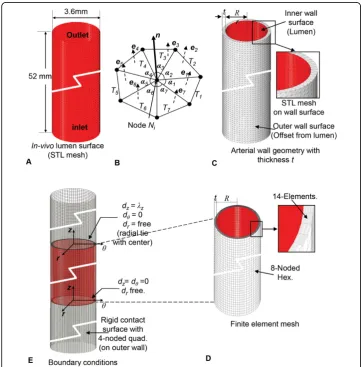
A straight arterial segment of a canine femoral artery of length of 52 mm, inner radius of 1.8 mm and thickness of 0.27 mm was adopted for this study [13]. This geometry is a simplified version of the tapered femoral artery studied by Sinha-Roy et al, [13]. In this study, the taper due to the reduction of 0.1 mm radius from the inlet to the outlet over the 52 mm length (angle of 0.11°) was neglected.
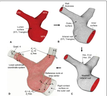
The lumen geometry is shown in Figure 1A, which can be obtained using image reconstruction if a patient-specific case is used. The outer wall surface of the artery was obtained by offsetting the lumen surface by computing an angle weighted normal
at each node of the stitched STL triangles (Figure 1B). The outward normal direction was computed by,
N=
k
αkek
k
αk
, (1)
where,e1,e2, ... are the unit normals of thek individual triangles,T1,T2, ... at a node of the STL mesh. The angles a1, a2, ... are the included angle for these triangles (Figure 1B). The position vector, R, of a node on the outer wall surface was calculated from the corresponding position, r, of the node on the inner wall by:
R=r−tnˆ. (2)
where,tis thein-vivowall thickness and nˆ=NN is the unit normal vector at the node (Figure 1B). The resulting wall geometry was obtained as a mesh of surface trian-gles as shown in Figure 1C. The wall geometry was meshed with 4-noded linear hexa-hedral elements with 15 elements across thickness (Figure 1D). This meshed geometry was used to construct the finite element model for the inverse algorithm described below (Figure 1E).
Arterial wall material property
The arterial wall material was modeled as homogeneous, incompressible, isotropic material of hyperelastic type. The constitutive equations for the wall material were derived using the generalized Mooney-Rivlin strain energy density function, W, of orderN= 2
W= N
p,q=0
p+q=1
Cpq(I1−3)p(I2−3)q (3)
with invariantsI1andI2[1,2,26,27]. The material constants:C10= 1.157 × 10⁻³N/mm2,
C01= -0.314 × 10⁻³N/mm2,C20= 13.689 × 10⁻³N/mm2,C11= 7.942 × 10⁻³N/mm2, and
C02= 4.433 × 10⁻³N/mm2were obtained by nonlinear least square curve-fitting using the circumferential stress-strain data for the canine femoral artery obtained by Attinger, 1968 [28]. The plot of computed Cauchy stresses verses stretch in the circumferential direc-tion is shown in Figure 2A along with the experimental data. Since the material model is isotropic, the longitudinal stress versus strain plot for the material will be same as the circumferential plot (Fit:Circumferential, Figure 2A). The experimentally obtained longitudinal stress versus stretch data is also plotted in the same figure for comparison. The material testing by Attinger (1968) was performed with an excised tubular-shaped sample of the artery [28]. Therefore, the constitutive model (Eq. 3), obtained by model-fitting the test data can be directly adopted for the cylindrical arterial geometry used in this study. It may also be noted that the cylindrical arterial specimen has resi-dual stresses. Therefore, the resiresi-dual stresses are indirectly included through the mate-rial model.
magnitude of strain energy density,W, atlz=lθ= 1 is 0.0 (Figure 2B). This demonstrates the validity of the material model obtained by curve-fitting.
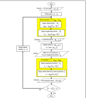
Inverse algorithm: load-free and pre-stressed wall geometry
The optimization-based inverse algorithm (Figure 3) was implemented using two operators: a) Shrink (S), and b) Fit (F). The operators, Sand F, were based on two basic modes of wall deformation: radial deformation,cRSand longitudinal deformation,
cLS, as described below. The shrink operator, S, shrinks the arterial geometry in the
radial direction by δr, with the deformation operator cRS, followed by a longitudinal
shrinking byδl, using the deformation operator cLS. The fit operator, F, was
imple-mented to apply the in-vivolongitudinal stretch,δIand then apply mean arterial
pres-sure,pI(Figure 3).
Longitudinal deformations,cLS
artery, whereas a solution with δl < 0 shrinks the artery radially. Since the sliding
con-tact computation projects the arterial nodes on the rigid concon-tact surface, this surface was extended at the inlet, as well as the outlet (Figure 1E), for ensuring a robust con-vergence of the contact solve.
Radial deformations,cRS
The radial deformation operator performs radial expansion (stretch) or contraction (shrink) of the artery. The radial deformation can be performed in two ways: 1) a geometrical scaling by offsetting the nodes in the normal direction, nˆ (Eq. 2) or 2) by expanding the arterial wall by applying a mean arterial pressure, pI. No wall stres-ses are produced in the process of radial deformation by geometrical scaling. How-ever, stresses are generated in the process of radial expansion under the pressure load, pI. In a manner similar to cLS, the radial deformation is denoted by:cRS(X,a)
and its inputs are the arterial configuration represented by X and a real numbera. The parametera can be pressure (pI) in the case of pressure induced deformation, or it can be a real number δr for the geometric scaling operation. The pressure induced
radial deformation can only result in a radial expansion of the arterial wall. Applying a negative value of pressure at the inner wall is not feasible as it will lead to material instability. For geometric deformation by scaling, cRS can expand the artery radially
by applying a radial stretch, δr,δr> 0, or it can shrink the artery radially by applying,
δr < 0.
Inlet and outlet constraints
At each inlet and outlet cross-section, a local cylindrical coordinate system, (dr,dθ,dz), was created with its origin at the center of the cross-section. The coordinate system axis, dzwas defined normal to the cross-sectional plane (Figure 1E). The nodal con-straints for the nodes on the cross-section plane were defined with respect to this local cylindrical coordinate system. A reference node was created at the origin of the coordi-nate system and was held fixed to prevent any rigid body motion (Figure 1E). To allow the radial wall deformation due to pulsatile pressure, all nodes on the inlet and outlet were allowed to move in the radial direction from the reference node. The displace-ment of those nodes in the dzdirection was prevented only at the inlet. At the outlets, motion of the nodes in the dzdirection was allowed in order to apply longitudinal shrink or stretch.
Inverse algorithm
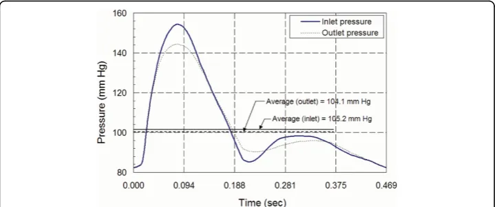
The inputs for the inverse algorithm are: 1) the unstressed in-vivoshape of the artery, 2) the mean in-vivoarterial pressure, pI, and 3) the in-vivoaxial stretch,δI. For the femoral artery, pIwas 104.1 mmHg andδI was considered to be 48% of the load-free artery length [4]. The inverse algorithm presented here, modifies the un-stressed in-vivo arterial geometry by performing the shrink and fit operations, resulting in new arterial configurations. To describe these configurations and their respective stress-states, a notation of A(x,s) has been used in which, xis used to denote a particular configuration, e.g.,xIforin-vivo andxLfor load-free, etc.; andsis used to represent a 3x3 stress tensor for symbolically denoting the non-zero stress-state of the configura-tion. Therefore,A(xI,0) is used to denote the un-stressedin-vivo arterial configuration, where0represents the 3 × 3 null tensor. The steps (Figure 3) of the inverse algorithm are as follows:
2. Apply shrink (S) to the unstressed in-vivoartery geometry, A(xI, 0). This is per-formed in two steps:
a. Apply radial shrink,cRSto thein-vivogeometry,A(xI,0), to radially shrink byδr.
That is:xRS =cRS (xI, δr), wherexIis a point on thein-vivo artery geometry, and
xRS, its mapping on the radially shrunk artery.
b. Apply longitudinal shrink,cLSto the artery geometry resulting in the step 2a.
That is:xL=cLS(xRS, δl), where xL is a point on the load-free artery after radial
and longitudinal shrink. The resulting shrunk artery geometry,A(xL,sL) has
stres-ses,sL.
3. Delete stresses, sL from A(xL, sL) to obtain A(xL, 0). This is a trial load-free geometry.
4. Apply fit (F) toA(xL, 0) obtained in step 3. This is also performed in two steps:
a. Apply longitudinal stretch,cLS to stretch theload-free geometry,A(xL,0) byδI.
That is:x1=cLS(xL,δI), wherex1is the location ofxLafter longitudinal stretch.
b. Apply radial expansion,cRS, by applying in-vivomean pressure,pI. That is:x = cRS(x1,pI), wherexis a point on the pre-stressed artery. The result is a trial
pre-stressedgeometry,A(x,s), with stresses, s.
5. Evaluate the least-square error function,ε:
ε=x−xI=
x−xI2, (4)
which is defined as the sum of the deviation of the nodal position of the nodes in the set Ω, between their location on the pre-stressed artery and their corresponding loca-tion, xI, in thein-vivoartery. For this study, Ωwas taken as the set of nodes on the outer surface of the arterial wall.
6. Stop the algorithm, if the value ofεis less than a pre-determined limit,L;
else, if ε>L, update,δr, andδlusing Nelder-Mead optimization algorithm and
pro-ceed to the Step-2. The value of Lwas assumed to be 0.5 in this study.
It may be noted in Step-4, described above, that the pre-stressed arterial geometry was computed as a part of the inverse algorithm. Therefore, the two sequential outputs of the converged algorithm are: a) a load-free arterial geometry (Step 3); and b) the corresponding pre-stressed geometry (Step 4).
Any geometrical shape matching-based inverse algorithm has two key operators: 1) an optimization operator(Step-6) to compute a trial load-free geometry and 2) a computa-tional mechanics operator(Step-2 and Step-4), to compute the deformed shape after the application of the in-vivopressure and longitudinal stretch. It is well established that arterial wall materials are incompressible in nature. In the computational mechanics operator, this incompressible behavior is incorporated through the material model. In the present study, this has been achieved by using incompressible hyperelastic Mooney-Rivlyn material. However, for a realistic simulation, theoptimization operatorwhich computes a trial load-free arterial shape, also needs to incorporate this incompressibility constraint. In this research, this was done through an additional volumetric constraint to preserve thein-vivoarterial volume during optimization iteration.
Implementation and convergence
Pulsatile pressure-flow response
The equations of motion for the arterial wall and blood-flow along with the boundary conditions are described in the previously published research by Konala et al., [29]. The pulsatile pressure-flow response of the arterial wall was computed by solving the coupled equations of wall deformation and the hemodynamic equations of blood flow using ADINA (ADINA R & D, Inc., Watertown, MA). The non-Newtonian blood was modeled as a Carreau fluid [30].
The dimensions of the load-free arterial geometry were obtained by the inverse method described above. An axisymmetric finite element model of the fluid and the structure was used for the pulsatile pressure-flow analysis [29]. The analysis was performed in two steps. In the first step, the load-free artery geometry, which was obtained in the Step 3 of the inverse algorithm, was pre-stressed by applyingin-vivolongitudinal stretched,δI, and the
meanin-vivoarterial pressure,pI. In the second step, the pulsatile pressure was applied to the pre-stressed artery. The pressure pulses,pin(t) andpout(t) were applied at the inlet and outlet, respectively (Figure 5), as normal surface tractions [13].
Results
The results are presented in three sections. First, the results for dimensions of the load-free and pre-stressed geometry computed by the inverse algorithm are presented.
Figure 4Algorithm convergence. Convergence of the inverse algorithm in terms of the objective function value and the number of function evaluation.
Then the stresses and strains in the pre-stressed arterial wall are presented. Finally, the arterial wall stresses under the combined pulsatile pressure load and arterial wall pre-stress are presented.
Load-free and pre-stressed arterial geometry
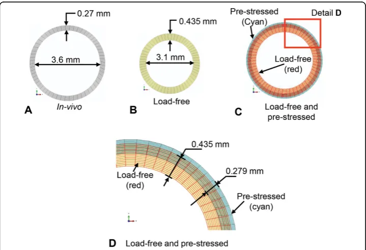
The cross-sectional dimensions of the load-free and pre-stressed arterial geometry for the femoral artery using the inverse algorithm are presented in Figure 6. The in-vivo artery dimensions are shown in Figure 6A. The load-free artery dimensions computed by the inverse algorithm are shown in Figure 6B. The dimensions of the pre-stressed artery obtained by applyingin-vivo longitudinal stretch and mean arterial pressure to the load-free geometry are shown in Figure 6C and 6D. For comparison, an image of the load-free geometry is also superimposed on the image of the pre-stressed artery.
The dimensions of the in-vivo, load-free and the pre-stressed artery are compared in Table 1. The length, inner diameter and thickness of the load-free arterial geometry calculated by the shrink-and-fit inverse algorithm are: 35.14 mm, 3.1 mm and 0.435 mm, respectively. The load-free artery length of 35.14 mm represents shrinkage of 32.4% from the in-vivo length of 52 mm. It also represents an axial stretch of 48% from the load-free length to thein-vivolength. The diameter change from the inner arterial wall, between the load-free artery (3.1 mm) and the in-vivoartery (3.6 mm) was 16.2%, whereas that for the outer arterial wall was 4.3%. The thickness of the load-free artery was 0.435 mm, which was 61% thicker than the in-vivo artery with thickness 0.27 mm.
The length, inner diameter and the thickness of the pre-stressed artery obtained by applying a mean arterial pressure and axial stretch of 48% to the load-free geometry were: 51.99 mm, 3.603 mm and 0.2685 mm, respectively. The pre-stressed arterial geo-metry shows a reasonable match with thein-vivoshape as is evident from the compari-son of the corresponding dimensions shown in Table 1. The difference in length between the in-vivoartery and the pre-stressed artery was 0.01 mm (0.019%). The inner wall diameter of the pre-stressed artery was within 0.004 mm (0.11%) of the in-vivo inner wall diameter of 3.6 mm. The difference in wall thickness between the in-vivoartery and pre-stressed artery was 0.0015 mm (0.37%).
The volume of the load-free as well as the pre-stressed artery was 169.90 mm3. This volume was calculated from the tessellated arterial geometry (Figure 2B). It was within 0.79 mm3 of the in-vivo volume of 170.69 mm3 since the optimization based inverse algorithm has preserved the material volume of the artery.
Stresses and strains in pre-stressed artery
The stress, strain and deformation results for the pre-stressed artery under the mean in-vivo pressure of 104.1 mmHg andin-vivo longitudinal stretch of 48% from the load-free length are presented in this section. The value of the stresses, strains and deforma-tions at the inner and the outer wall are tabulated in Table 2.
The radial stress (srr) varies from the value of 0.0136 N/mm2, at the inner wall, equal to the applied pressure, to 0.0 N/mm2on the outer wall surface (Table 2). The change in circumferential stress from the inner wall surface (0.127 N/mm2) to the outer wall sur-face (0.071 N/mm2) was 44%. Due to the nonlinear material property, the longitudinal stress also varied across the vessel thickness. The difference in the longitudinal stress between the inner (0.193 N/mm2) and the outer wall (0.140 N/mm2) was 27.8%. In the pre-stressed configuration, the circumferential stresses are lower in magnitude than the longitudinal stresses. At the inner wall, the circumferential stress (0.127 N/mm2) was 34% lower than the longitudinal stress (0.193 N/mm2). Similarly, at the outer wall, Table 1 Inverse algorithm results
In-vivo (I)
Load-free (inverse)
Pre-stressed
(P) %=
I−P
I
×100
Inner diameter (mm) Inlet 3.60 3.104 3.604 1.1 × 10⁻¹
Outlet 3.60 3.104 3.604 1.1 × 10⁻¹
Outer diameter (mm) Inlet 4.14 3.974 4.140 0.0
Outlet 4.14 3.974 4.140 0.0
Thickness (mm) 0.270 0.435 0.269 3.7 × 10⁻¹
Length (mm) 52.0 35.13 51.99 2.0 × 10⁻²
Volume (mm3) 170.69 169.90 169.90 4.6 × 10⁻¹
The dimensions of load-free and pre-stressed geometry calculated by the inverse algorithm.
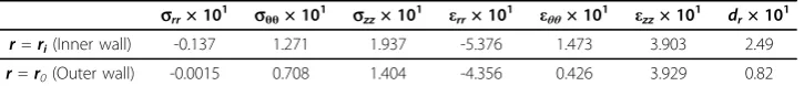
Table 2 Arterial wall stresses on inner and outer wall surface
srr× 101 sθθ× 101 szz× 101 εrr× 101 εθθ× 101 εzz× 101 dr× 101
r=ri(Inner wall) -0.137 1.271 1.937 -5.376 1.473 3.903 2.49
r=r0(Outer wall) -0.0015 0.708 1.404 -4.356 0.426 3.929 0.82
Stresses, logarithmic strains and radial deformation on the inner and outer arterial wall of the pre-stressed artery. Units for deformations are in mm and stresses in N/mm2
the circumferential stress (0.071 N/mm2) was 49% lower than the longitudinal stress (0.140 N/mm2).
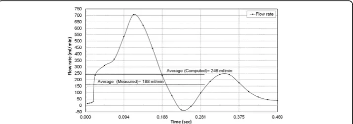
Pulsatile flow rate
The transient flow rate computed for the pre-stressed artery by applying the pulsatile pressure pulse is shown in Figure 7. The numerically computed time averaged flow rate, 246 ml/min, was 30% higher than the measured flow rate of 188 ml/min as reported by Sinha-Roy et al., [13], for the tapered femoral artery. The measured flow rate of 188 ml/min was obtained using Doppler flow wire for the tapered femoral artery. The difference between the computed and measured value could be because of Doppler measurements, which are based on average peak velocity (APV) and have been reported to register a lower flow rate than actual [31-33].
Wall stresses under pulsatile pressure load
The variation of the longitudinal and circumferential Cauchy stress over the cardiac cycle under the pulsatile inlet and outlet pressure pulse is presented in Figure 8. The time averaged value of Cauchy stress at the inlet in the longitudinal direction was 0.148 N/mm2, and that in the circumferential direction was 0.104 N/mm2. Therefore, for an in-vivo axial stretch of 48%, the time averaged longitudinal stress was 42.5% higher than the circumferential stress.
Due to the pulsatile flow, the time-averaged longitudinal stresses had a difference of 0.001 N/mm2 between the inlet (0.149 N/mm2) and the outlet (0.148 N/mm2). Between the inlet (0.104 N/mm2) and the outlet (0.101 N/mm2), the corresponding dif-ference in the circumferential stress was only 0.003 N/mm2. The peak stress in the cir-cumferential direction was 0.187 N/mm2 at the inlet and 0.168 N/mm2 at the outlet, which corresponded to the time instant of peak pressure (Figure 5). Therefore, as evi-dent from Figure 8, the overall time-variation of stress showed a similar trend between the inlet and outlet.
Discussion
The primary contribution of this study was the development of an inverse algorithm to calculate the in-vivoarterial pre-stress for a patient-specific artery. This algorithm was developed for a patient-specific arterial geometry. For the present study, the algorithm was tested using an idealized arterial wall geometry that was cylindrical in shape. Even
though this idealized geometry was axisymmetric, the algorithm was tested using a 3D cylindrical geometry. This was done to mimic the steps of a patient-specific case.
In addition to the idealized axisymmetric geometry, the algorithm was tested for a 3D patient-specific arterial geometry. This was done to test the proposed steps (Figure 3) as described in the methods section, for a patient-specific case. The intermediate steps of the inverse algorithm for a patient-specific artery are shown in Figure 9. Specifically, Figure 9A shows the lumen boundary, which in the patient-specific case will be obtained from image reconstruction. As shown in Figure 1A, for the straight artery case, this sur-face is simply a cylindrical sursur-face. Similarly, Figure 9B shows the arterial wall geometry obtained by adding wall thickness using nodal normal defined by Eq. 1. The correspond-ing wall geometry for the straight artery case (Figure 1C) was constructed by adaptcorrespond-ing the same procedure. Next, the finite element mesh used by the longitudinal and radial shrink operators for the patient-specific case is presented in Figure 9C, whereas Figure 1D shows the same for the straight artery. Finally, the boundary con-ditions and constraints imposed on the finite element mesh for the patient-specific case and the straight artery case are shown in Figure 9C and 1D, respectively. The complete pressure-flow analysis using blood-arterial wall interaction for such a patient-specific case will be presented in future.
The proposed algorithm simplified the inverse optimization problem to a two variable problem involving radial and axial deformation. This helped in substantially reducing the number of optimization variables from positions of each node to just two variables. Moreover, the incompressibility of arterial material was incorporated in the inverse opti-mization as a volumetric constraint; which preserved thein-vivoarterial volume during optimization iterations. The performance and robustness of the algorithm for patient-specific case needs to be tested with realistic artery geometry. For example, the algo-rithm employed a longitudinal wall deformation operator to shrink or stretch the arterial wall. The operator used sliding contact on a rigid contact surface, without contact separation, to deform the wall while not altering itsin-vivoarterial shape. However, for a patient-specific case, the accuracy and performance of the contact algorithm is expected to be influenced by the complex and tortuous 3D wall shape.
In the implementation of the inverse method, the Nelder-Mead optimization algo-rithm was utilized for solving the non-linear least square minimization problem. One of the drawbacks of the Nelder-Mead algorithm is its slow convergence near the
optimal solution. In addition to that, the convergence of Nelder-Mead to an optimal solution has not been proven mathematically. Other researchers have typically used the Levenberg-Marquardt (LM) algorithm for inverse computation. However, the advantage of Nelder-Mead is that it is a derivative free algorithm, whereas LM requires computation of derivatives. The computation of the derivatives can be expensive when a finite element solution is required for the evaluation of the objective function.
In the test with the idealized straight arterial geometry, the proposed inverse algo-rithm was found to converge to an acceptable solution within 20 to 25 evaluations of the objective function (Figure 4). However, as stated above, the convergence and robustness of the algorithm needs to be tested for a real patient-specific case.
The validity of the load-free geometry computed by the inverse algorithm was assessed by two criteria: 1) the geometrical match between the dimensions of the pre-stressed artery and thein-vivoartery, and 2) the change in diameter between the load-free artery and the pre-stressed artery. The first criterion is the necessary condition for a valid inverse solution. The second criterion is also important which is discussed here. It is
Figure 9Application of the inverse algorithm to a patient-specific artery. Intermediate steps of the inversealgorithm. A) Lumen surface in form of triangular mesh of STL triangles obtained by geometry reconstruction. B) Arterial wall geometry in form of STL-mesh of surface triangles. C) Finite element mesh of the wall geometry using 8 node (or 20 node) hexahedral elements. D) Constraints imposed on the arterial wall motion in each shrink and fit iteration. Rigid contact surface superimposed on the outer arterial wall surface and extended at the ends, to maintain arterial shape during the longitudinal (axial) shrink or stretch operation. Contact surface meshed with 4-noded quadrilateral elements. Only in-plane radial motion indr-dθplane allowed for the nodes of the inlet and outlet surfaces. Additionally, nodes of
possible to obtain a solution of the inverse problem satisfying the first criteria even if inaccurate arterial wall material properties are specified in the computational model. However, under such a scenario the deformation of the pre-stressed artery from the load-free configuration may not be accurate. For example, if the arterial wall material property is erroneously specified to be softer than what is actually observed, the defor-mation of the artery from the load-free to the pre-stressed configuration will be large. Excessive diameter changes between the calculated load-free geometry and the pre-stressed geometry will imply inaccurate load-free geometry. Ideally, the diameter change should match with thein-vivomeasurements. For the femoral artery in the present study, the change in the outer diameter was 4.3% between the load-free (3.97 mm) and pre-stressed artery (4.14 mm). The corresponding change in the inner diameter was 14%. This was similar to the 5% outer diameter change reported by Huang et al., [5], for a human carotid artery using a direct method (based on trial and error procedure). Simi-larly, a change of 19% in the inner diameter of a porcine left anterior descending (LAD) artery was reported by Hamza et al., [7].
It may be noted that the pre-stresses in an arterial wall segment are the result of equilibrium of the wall segment (in the time averaged sense) under the applied stresses and stretch. This equilibrium is primarily a balance between the different stress com-ponents caused by the arterial pressure and tethering, along with the shear stresses due to the blood flow, in relation to the stretch ratios in the axial, circumferential and radial directions. Therefore, as indicated by Raghavan, et al., [34], some deviations in the arterial wall material property values do not significantly affect the results of the wall pre-stress. However, specification of significantly inaccurate material properties may result in an incorrect computation of the load-free arterial geometry.
The time-averaged flow rate computed with the pulsatile pressure was 30% higher than the measured value of 188 ml/min as reported by Sinha-Roy et al., [13]. The poten-tial under-measurement than actual arterial flow rate by the Doppler flow wire, which measure flow rate based on APV could have contributed to this difference [31-33].
The magnitude of the average circumferential and longitudinal stress in the artery has been reported to depend on the value of the longitudinal stretch applied to an un-tethered and unloaded, ex-vivo artery. For porcine LAD, Zhang et al., [35], have reported lower magnitude of the average stress in the longitudinal direction compared to the circumferential direction when the axial stretch was less than 40%. They report that longitudinal stresses exceed circumferential stresses for axial stretch ratios greater than 1.4 (i.e., 40% stretch from load-free length). The present study shows a develop-ment of higher stresses in the longitudinal direction than circumferential, when the artery is subjected to an in-vivolongitudinal stretch of 48% from its load-free length. Specifically, under the pulsatile pressure, the mean stress in the longitudinal direction was 42.5% higher than the stress in the circumferential direction.
[8], for coronary arteries and Guo et al., [6], for coronary arteries, as well as veins. Guo et al., [6] study have also shown the dependence of in-vivoaxial stretch on the vessel diameter. It is possible that the axial stretch of 48% for the diameter of the femoral artery evaluated in this study may need further investigation.
Conclusions
In this study, a methodology has been developed to incorporate the arterial wall pre-stress in wall-blood flow interaction computation under pulsatile pressure. An optimi-zation-based inverse algorithm has been developed and tested to incorporate arterial wall pre-stresses in the computational model. This algorithm was used to compute the load-free arterial geometry from thein-vivoarterial wall shape, axial stretch and mean arterial pressure. For the canine femoral artery, the resulting pre-stressed artery geo-metry, obtained by subjecting the computed load-free geometry to in-vivopressure and longitudinal stretch, was within 0.0015 mm of the in-vivogeometry. The inverse algo-rithm has been designed to handle patient-specific cases. However, further testing is required for a patient-specific case with: a) the realistic material property, and b) an accurate measurement of the in-vivolongitudinal stretch.
Under pulsatile pressure and the in-vivo axial stretch of 48% from the load-free length, the arterial stress in the longitudinal direction was found to be 42.5% higher than those in the circumferential direction. This could be the result of either the rela-tively higher in-vivo stretch (48% of load-free length) considered in our computation or the use of an isotropic material model for the arterial wall material, rather than an anisotropic material formulation.
Nomenclature
x = a point of the pre-stressed artery. xI= a point of thein-vivoartery.
xL= a point of the load-free artery.
δr= radial deformation computed by optimization algorithm.
δl= length of longitudinal or axial stretch (or shrinking) computed by the
optimiza-tion algorithm. δI=in-vivoaxial stretch.
pI= meanin-vivopressure. cRS= radial deformation operator.
cLS= longitudinal or axial deformation operator.
S= shrink operator to shrinks the arterial geometry in the radial and axial direction. F = fit operator to deform artery by applying the in-vivolongitudinal stretch and
meanin-vivopressure.
sL= residual stresses in the load-free artery; a 3 × 3 tensor.
s= stresses in pre-stressed artery; a 3 × 3 tensor. 0= zero stress state (at all points); a 3 × 3 null tensor. A(xI,0) =in-vivoarterial geometry without any stress. A(xL,sL) = load-free arterial geometry with stresses,sL. A(xL,0) = load-free arterial shape with stresses deleted. A(x,s) = pre-stressed artery with stresses,s.
Disclosure
The method presented in this manuscript is covered by a pending provisional patent (U.S. Serial No. 62/029028 dated July 25, 2014).
Competing interests
The authors declare that they have no competing interests.
Authors’contributions
AD did the study design, developed the inverse program, performed numerical calculations and analyzed results, and drafted the manuscript. AP contributed to technical discussion, meshing of the arterial wall geometry and reviewed the manuscript. RKB’s contributions include study design, data interpretation, and approval of the final manuscript. MT was involved in technical discussion. All authors read and approved the final manuscript.
Acknowledgements
This work was partially supported by an internal funding provided by the College of Engineering and Applied Science at the University of Cincinnati.
Declarations
Publication charge for this article was paid with funding from Cincinnati Children’s Hospital Medical Center (CCHMC). This article has been published as part ofBioMedical Engineering OnLineVolume 14 Supplement 1, 2015:
Cardiovascular Disease and Vulnerable Plaque Biomechanics. The full contents of the supplement are available online at http://www.biomedical-engineering-online.com/supplements/14/S1
Authors’details 1
Department of Mechanical and Materials Engineering, University of Cincinnati, Cincinnati, OH 45221, USA.2Cincinnati Children’s Hospital Medical Center, The Heart Institute, 3333 Burnet Avenue, Cincinnati, OH 45219, USA.
Published: 9 January 2015
References
1. Fung YC:Biomechanics: mechanical properties of living tissuesNew York: Springer-Verlag; 1981.
2. Holzapfel GA, Ogden RW:Biomechanics of soft tissue in cardiovascular systemsWien; New York: Springer; 2003. 3. Holzapfel GA, Ogden RW:Mechanics of Biological Tissue.InBook Mechanics of Biological Tissue. Volume xii.City:
Springer; 2006:522.
4. Van Loon P:Length-force and volume-pressure relationships of arteries.Biorheology1977,14:181-201.
5. Huang X, Yang C, Yuan C, Liu F, Canton G, Zheng J, Woodard PK, Sicard GA, Tang D:Patient-specific artery shrinkage and 3D zero-stress state in multi-component 3D FSI models for carotid atherosclerotic plaques based on in vivo MRI data.Mol Cell Biomech2009,6:121-134.
6. Guo X, Liu Y, Kassab GS:Diameter-dependent axial prestretch of porcine coronary arteries and veins.J Appl Physiol (1985)2012,112:982-989.
7. Hamza LH, Dang Q, Lu X, Mian A, Molloi S, Kassab GS:Effect of passive myocardium on the compliance of porcine coronary arteries.Am J Physiol Heart Circ Physiol2003,285:H653-660.
8. Algranati D, Kassab GS, Lanir Y:Why is the subendocardium more vulnerable to ischemia? A new paradigm.Am J Physiol Heart Circ Physiol2011,300:H1090-1100.
9. Horny L, Adamek T, Kulvajtova M:Analysis of axial prestretch in the abdominal aorta with reference to post mortem interval and degree of atherosclerosis.Journal of the mechanical behavior of biomedical materials2014, 33:93-98.
10. Horny L, Adamek T, Vesely J, Chlup H, Zitny R, Konvickova S:Age-related distribution of longitudinal pre-strain in abdominal aorta with emphasis on forensic application.Forensic science international2012,214:18-22.
11. Huang X:In-vivo MRI-Based Three-Dimensional Fluid-Structure Interaction Models and Mechanical Image Analysis for Human Carotid Atherosclerotic Plaques.PhD DissertationWorcester Polytechnic Institute; 2009.
12. Tang D, Yang C, Zheng J, Woodard PK, Saffitz JE, Sicard GA, Pilgram TK, Yuan C:Quantifying effects of plaque structure and material properties on stress distributions in human atherosclerotic plaques using 3D FSI models. J Biomech Eng2005,127:1185-1194.
13. Sinha Roy A, Back LH, Banerjee RK:Evaluation of compliance of arterial vessel using coupled fluid structure interaction analysis.Mol Cell Biomech2008,5:229-245.
14. Konala BC, Das A, Banerjee RK:Influence of arterial wall-stenosis compliance on the coronary diagnostic parameters. Journal of Biomechanics2011,44:842-847.
15. Lu J, Zhou X, Raghavan ML:Computational method of inverse elastostatics for anisotropic hyperelastic solids. International Journal for Numerical Methods in Engineering2007,69:1239-1261.
16. Govindjee S, Mihalic PA:Computational methods for inverse deformations in quasi-incompressible finite elasticity. International Journal for Numerical Methods in Engineering1998,43:821-838.
17. Speelman L, Bosboom EM, Schurink GW, Buth J, Breeuwer M, Jacobs MJ, van de Vosse FN:Initial stress and nonlinear material behavior in patient-specific AAA wall stress analysis.J Biomech2009,42:1713-1719.
18. Raghavan ML, Ma B, Fillinger MF:Non-invasive determination of zero-pressure geometry of arterial aneurysms. Ann Biomed Eng2006,34:1414-1419.
20. de Putter S, Wolters BJ, Rutten MC, Breeuwer M, Gerritsen FA, van de Vosse FN:Patient-specific initial wall stress in abdominal aortic aneurysms with a backward incremental method.J Biomech2007,40:1081-1090.
21. Bols J, Degroote J, Trachet B, Verhegghe B, Segers P, Vierendeels J:A computational method to assess the in vivo stresses and unloaded configuration of patient-specific blood vessels.Journal of Computational and Applied Mathematics2013,246:10-17.
22. Lu J, Zhou X, Raghavan ML:Inverse method of stress analysis for cerebral aneurysms.Biomech Model Mechanobiol 2008,7:477-486.
23. Gee MW, Reeps C, Eckstein HH, Wall WA:Prestressing in finite deformation abdominal aortic aneurysm simulation. J Biomech2009,42:1732-1739.
24. Hsu M-C, Bazilevs Y:Blood vessel tissue prestress modeling for vascular fluid-structure interaction simulation.Finite Elements in Analysis and Design2011,47:593-599.
25. Lu J, Zhou X, Raghavan ML:Inverse elastostatic stress analysis in pre-deformed biological structures: Demonstration using abdominal aortic aneurysms.J Biomech2007,40:693-696.
26. Holzapfel GA:Nonlinear solid mechanics: a continuum approach for engineeringChichester; New York: Wiley; 2000. 27. Humphrey JD, Na S:Elastodynamics and arterial wall stress.Ann Biomed Eng2002,30:509-523.
28. Attinger FM:Two-dimensional in-vitro studies of femoral arterial walls of the dog.Circ Res1968,22:829-840. 29. Konala BC, Das A, Banerjee RK:Influence of arterial wall compliance on the pressure drop across coronary artery
stenoses under hyperemic flow condition.Mol Cell Biomech2011,8:1-20.
30. Cho YI, Kensey KR:Effects of the non-Newtonian viscosity of blood on flows in a diseased arterial vessel. Part 1: Steady flows.Biorheology1991,28:241-262.
31. Doriot P, Dorsaz P, Dorsaz L, Chatelain P:Accuracy of coronary flow measurements performed by means of Doppler wires.Ultrasound in medicine & biology2000,26:221-228.
32. Doucette JW, Corl PD, Payne HM, Flynn AE, Goto M, Nassi M, Segal J:Validation of a Doppler guide wire for intravascular measurement of coronary artery flow velocity.Circulation1992,85:1899-1911.
33. Jenni R, Matthews F, Aschkenasy SV, Lachat M, van Der Loo B, Oechslin E, Namdar M, Jiang Z, Kaufmann PA:A novel in vivo procedure for volumetric flow measurements.Ultrasound in medicine & biology2004,30:633-637.
34. Raghavan ML, Vorp DA:Toward a biomechanical tool to evaluate rupture potential of abdominal aortic aneurysm: identification of a finite strain constitutive model and evaluation of its applicability.J Biomech2000,33:475-482. 35. Zhang W, Herrera C, Atluri SN, Kassab GS:The effect of longitudinal pre-stretch and radial constraint on the stress
distribution in the vessel wall: a new hypothesis.Mechanics & chemistry of biosystems: MCB2005,2:41-52. 36. Guo X, Kassab GS:Variation of mechanical properties along the length of the aorta in C57bl/6 mice.Am J Physiol
Heart Circ Physiol2003,285:H2614-2622.
doi:10.1186/1475-925X-14-S1-S18
Cite this article as:Daset al.:Pulsatile arterial wall-blood flow interaction with wall pre-stress computed using an inverse algorithm.BioMedical Engineering OnLine201514(Suppl 1):S18.
Submit your next manuscript to BioMed Central and take full advantage of:
• Convenient online submission
• Thorough peer review
• No space constraints or color figure charges
• Immediate publication on acceptance
• Inclusion in PubMed, CAS, Scopus and Google Scholar
• Research which is freely available for redistribution