Robust Fault Diagnosis for Discrete-Time Switched System with Unknown State Delays Subject to Component Faults

(1)

Information Technology and Control 2019/1/48 146

Robust Fault Diagnosis for

Discrete-Time Switched System

with Unknown State Delays

Subject to Component Faults

ITC 1/48

Journal of Information Technology and Control

Vol. 48 / No. 1 / 2019 pp. 146-159

DOI 10.5755/j01.itc.48.1.20162

Robust Fault Diagnosis for Discrete-Time Switched System with Unknown State Delays Subject to Component Faults

Received 2018/07/12 Accepted after revision 2019/01/22

http://dx.doi.org/10.5755/j01.itc.48.1.20162

Corresponding author: [email protected]

Haigang Zhang

Tianjin Key Lab for Advanced Signal Processing; Civil Aviation University of China; Tianjin Dongli District, Tianjin North Highway 2898, China; e-mail: [email protected]

This paper investigates the problems of fault detection and diagnosis in a class of discrete-time switched sys-tems with unknown state delay against component faults. The component fault, also called the multiplicative fault or loss of actuator effectiveness, is a common type of operation fault for switched systems, which has been paid more attention. In this paper, the learning observers (LOs) technology are proposed to reconstruct both the system state and component faults. The proposed LOs technique is also extended to the system with un-known time delay and external disturbance. The sufficient conditions for the convergence of the output of LOs and the uniformly ultimately boundedness of the reconstructed errors are proved by the switched Lyapunov function and H∞ technique. The proposed fault reconstruction strategy has certain tolerance for fault types,

which is effective for both slow and fast time-varying faults by adjusting the iteration step size. In the simula-tion parts, three kinds of fault signals are taken into considerasimula-tion to verify the effectiveness and robustness of the proposed method.

KEYWORDS: Fault Diagnosis, Switched System, Unknown State Delay, Lyapunov Function.

1. Introduction

With the increasing complexity of modern industrial systems and higher pursuit of system performance, fault diagnosis is an important and challenging prob-lem in many practical systems, such as chemical

(2)

147 Information Technology and Control 2019/1/48

diagnosis works have been published in several excel-lent papers and books [3, 5, 14, 15, 17, 23, 26]. Among these approaches, the most commonly used one is first to design the observers or filters to reconstruct the fault signal or residual signal, and then generate an alarm when the residual function is larger than the threshold or the fault reconstruction signal is not zero [18]. Recently, several physical systems present hybrid be-haviors [6, 19]. Wherein, the switched systems play an important role in industrial process and have drawn more and more attention for the stability and control-lability research [5]. A generalized switched system is composed of subsystems with their own parameters subject to a specific rule orchestrating the switching law among the various subsystems. The motivation of studying switched systems drives from the facts that many physical scenes exhibit the switching features among multi-models.

Because of the increasing demand for the operational safety refer to switched systems, the research about fault diagnosis of switched systems has been a hot top-ic [7]. Hwang et al. [12] introduced three types of fault in the field of model-based systems, including actua-tor fault, sensor fault and component fault or loss of effectiveness fault. The actuator fault and sensor fault are also called the additive fault, because they have an additional relationship with the original system state. There are many excellent fault diagnosis methods for additive faults in switched systems. In [4], a multiple Lyapunov function approach was employed for fault detection and diagnosis in switched systems. Then the switched Lyapunov function approach was first applied in stability analysis of switched systems [7]. Wang et al. [20] designed a fault filter for the actuator fault and sensor fault based on H∞ performance index.

Hespanha et al. [11] applied the average dwell time technology to conduct stability analysis for switched systems, while Zhang et al. [23] converted the fault detection problems into an H∞ filtering problem by

using the average dwell time technology. Du et al. [8] adopted the asynchronous switched approach in switched systems to reconstruct the additive faults. Compared with the actuator and sensor faults, the component faults or loss of effectiveness faults can also be called the multiplicative faults, which can weaken system input performance, and destroy the stability. It is necessary to design fault diagnosis strat-egy for component faults in switched systems. There

are relatively fewer research results for the switched systems with component faults. He et al. [10] designed a fault detection filter for a more general sensor fault, including the loss of effectiveness, the outage and the drifted fault in switched systems. The effectiveness of sensor was decayed in a certain proportion, and the attenuation rate was assumed to be a constant. Rodrigues et al. [16] proposed a fault tolerant control model for switched systems with component faults. However, the fault signal was set to be constant or slow time-varying. The component faults are multiplied with the actuator and sensor, which is the main reason why it is difficult to design the fault diagnosis method. In this paper, the learning observer technology is ap-plied to make reconstruction for the component faults in switched systems, which is a new attempt.

As is well-known, time-delay phenomenon is very common in many real physical systems, such as air pollution system and chemical process etc. [23]. It would often cause the instability and poor perfor-mance of the switched systems. There are some works about fault diagnosis taking time-delay phenomenon into consideration [20, 22]. Wang et al. [20] proposed a robust fault detection method for switched linear sys-tems with state delay. Yu et al. [22] presented a fault detection frame for discrete-time switched systems with distributed delays. However, the existing mod-els were only for additive faults. In addition, the delay time was known in advance. It should be mentioned that in our previous work [25], we designed an adap-tive fault diagnosis model for continuous time-delay repetitive systems subject to sensor fault, where the delay time was known in advance. In this paper, the unknown time-delay element is taken into consider-ation. A relatively slack restriction for delay time with known upper and lower bounds improves the gener-alization performance of fault reconstruction model. In this work, a fault diagnosis method based on LOs against the component faults for switched systems is proposed. It can handle the task of fault diagnosis for more complex systems, even with unknown de-lay time and external disturbance. Compared with the existing works for the constant faults or slowly time-varying faults, the proposed method is effec-tive for relaeffec-tively fast time-varying faults. By using the switched Lyapunov function and H∞ technique,

(3)

inequalities (LMIs). Finally, the simulation results for three forms of loss of actuator effectiveness faults demonstrate the feasibility of this scheme. To simpli-fy, the contributions of this paper can be summarized as follows:

1 The LOs are employed in switched systems against

component faults, which is a new attempt.

2 The time-delay element and external disturbance

are taken into consideration in the fault diagnosis model. A more relaxed bounded constraint for de-lay time is assumed, which leads to the proposed LOs having better generalization performance.

3 The proposed fault reconstruction strategy has

certain tolerance for fault types. It is still valid for fast time-varying faults.

The rest of the paper is organized as follows. In Sec-tion 2, the descripSec-tion for a generalized switched sys-tem is presented and the problems are formulated. Section 3 is the main part of this paper, which pres-ents the robust design of LOs. Simulation results are carried out in Section 4 and conclusions are drawn in Section 5. Section 6 is the appendix, where the proofs of the theorems are presented.

Notations: The notations used throughout the paper are normative. _AT_,_A−1_,_λ_{( )}_A _and _A _{are the symbols}

to denote, respectively, the transpose, the inverse, the eigenvalues and the Euclidean norm of any square matrix A. Particularly, λ_max( )A and λ_min( )A present the maximum and minimum eigenvalues of A. We use A>0

(

A<0

)

to denote that A is positive (nega-tive) defined and I to denote the identity matrix with an appropriate dimension. _∞ represents the infini-ty norm of any vector. The symbol * means the sym-metric terms in some matrices.

2. System Description and Problem

Formulation

We consider the following discrete-time switched system

( ) ( ) ( )

( 1) ( ) ( ) ( )

( ) ( )

k k

k

x k A x k B f k u k

y k C x k

σ σ

σ

+ = +

= 



 , (1)

where _{x k}

( )

_∈_Rm_,_{u k}

_{( )}

_∈_Rn_and_{y k}

_{( )}

_∈_Rp_{are the}

state, control input and output, respectively. Diago-nal matrix f k

( )

=diag f k

{

₁

( )

, ,⋅⋅⋅ f k_n

( )

}

represents the component faults with f k_i

( ) (

∈ 0,1

]

. Specifical-ly, when f k_i

( )

=1, the ith actuator runs fault-freely; if 0< f k_i

( )

<1, partial effectiveness of the actuator is lost; and f ki

( )

=0 means that the actuator has no effectiveness in the system totally. σ is the switching rule which takes the values in the finite set ℵ: 1, ,

{

⋅⋅⋅N

}

, where N is the number of subsystems. It is assumed that σ

( )

k is dependent on k or xk, or other

switch-ing rules at an arbitrary discrete time k. Aσ, Bσ, and

Cσ are of appropriate size constant known matrices.

Since f k

( )

is a diagonal matrix, the switched system can be rewritten as follows

( )

_{( )}

( )

_{( )}

( )

+1 _k _k _{k k}

k

x k A x k B U F

y k C x k

σ σ σ

= +

= 



 , (2)

where U_k =diag u

{

₁, ,⋅⋅⋅u_n

}

and Fk =f₁, ,⋅⋅⋅ fnT. .The fault signals are presented by a column vector, which is suitable for the following analysis and the proofs of the convergence theorems.

Assumption 1: The switching rule σ

( )

k is available at each sampling time k. Additionally, only one sub-system is active each time.

In most case, the switching signal is not known be-forehand, and that means one can not know in ad-vance the distribution of conversion signals. How-ever, the instantaneous value of switching signals is available. Thus, the design of observer modes will be modified with the change of switching signals. Some similar operations are shown in [2, 20].

Here we introduce the switching signal function as

( )

k 1

( )

k , , n

( )

k T

ξ =_ξ ⋅⋅⋅ξ _ , where ξ_i

( )

k Z: + _→

{ }

0,1

and

( )

1

1 N

i i

k

ξ =

=

∑

, k Z_∈ +_.

( )

₁

i k

ξ = means that the i

th subsystem is active at kth sampling step, while it is out of operation when ξ_i

( )

k =0. Then one can re-write the switched system as

( )

(

( )

)

( )

( ) ( )

1

+1 N _i _i _{i k k}

i N

i i

i

x k k A x k BU F

y k k C x k

ξ

=

= 

+

= 

    

∑

(4)

Assumption 2: The system control input u k

( )

is norm-bounded, u k

( )

≤u_max.

Assumption 2 says that the control input is bound-ed, which is reasonable for a system running in the normal operating environment. Additionally, the ob-servability is another reasonable hypothesis for the design of LOs in the following sections.

This paper aims to establish a fault diagnosis model to reconstruct the component faults F_k. The model should not only guarantee the convergence speed, but also be applied in many kinds of fault types. In addi-tion, it should be suscesful to deal with time-dalay phenomenon and externel disturbance.

3. Fault Reconstruction based on LOs

3.1. Design of Learning Observers

In this subsection, a novel fault reconstruction meth-od for the above switched system is presented. The corresponding LOs are established as

( )

(

( )

)

( ) ( )

(

)

( )

( ) ( )

(

)

1

1 2

ˆ

ˆ +1 ˆ

ˆ +

ˆ

,

ˆ

ˆ ˆ

N

i i i k k

i N

i i

i

k k

x k k A x k BU F

L y k y k

y k k C x k

F K F τ K y k y k

ξ

=

= −

 

= __ + __

 − 

 

=

= + −

            

∑



(4)

where x kˆ

( )

and y kˆ

( )

are the estimations of sys-tem state and output, respectively. Fˆk represents

the reconstructed fault of loss of actuator effective-ness updated by both its previous information at the sampling step k−τ and current output error.τ is the updating interval. K₁ is a diagonal matrix, that is,

{

}

1 1, , n

K =diag k ⋅⋅⋅k with k_i∈

(

0,1 ,

]

i∈ ⋅⋅⋅

{

1, , ,n

}

and

( )

1

, N

i i

i

L ξ k L

=

∑



( )

2 2

1

. N

i i

i

K ξ k K

=

∑



1,

K Li and K2i

would be selected later.

Define the system state-estimation error, out-put-estimation error and fault-estimation error as e k_x

( ) ( ) ( )

=x k −x kˆ ,e k_y

( )

=y k

( ) ( )

−y kˆ and

( )

ˆ .

F k k

e k =F F− In order to drive the fault recon-struction error less restrictively and reasonably, the following assumption is necessary.

Assumption 3: Denote Fk =F K Fk− 1 k−τ and assume

k

F _{is norm-bounded, such that}

k f

F ≤κ _.

Assumption 3 shows a relatively loose restriction compared with other works for fault diagnosis, where norm-bound condition of fault signal or its derivative is necessary. The restriction of norm-bound of the de-rivative of faults means that the corresponding faults are time-varying slowly, which is removed in this pa-per. The proposed LOs can deal with broader fault signals, including slowly and fast time-varying ones. Since 0< f_i ≤1, i=1,2, ,⋅⋅⋅n, the upper bound of

( )

F k _{can be calculated easily, such as}

1

f K

κ = + . Remark 1: The choice of K1 and τ is generally based

on human experience. K1 approximates the identity

matrix with proper dimension. It presents the influ-ence level of the historical reconstructed signal on the current one. A relatively larger value of K₁ means more information in the historical reconstructed signal is preserved, while less information is retained with rel-atively smaller value of K₁. In general, the value of τ

is determined according to the fault signal. When deal-ing with the fast time-varydeal-ing signal, τ should be suf-ficiently small. On the contrary, τ can be chosen as a larger interval if the fault signal is slow time-varying. Define the state error e kx

( )

, output error e ky

( )

and

fault error e k_F

( )

as

( ) ( ) ( )

( )

ˆ =

ˆ

= .

ˆ =

y

F x

k k

e k x k x k e k y k y k

e k F F

 ₋

 ₋

 

− 

(5)

Then one can get the following dynamic equations

( )

(

_{( )}

) ( )

( )

(

)

( )

1

2 1

+1 N i i i x

x i

i k F i

N

y i i x

i

F F

N

i i i x k

i

A L C e k

e k k

BU e k

e k k C e k

e k K e k

k K C e k F

ξ

τ

ξ

=

  − 

=  



_₊ _

 

 

 ₌

 

 ₌ _{− −}

 

 ₊



∑



.

(5)

3.2. Parameter Configuration of LOs

Here the analysis of LOs is presented. In order to fa-cilitate and simplify the proof, the matrix B_i is omit-ted. The convergence condition is presented in the following theorem, whose proof is shown in Part A in the appendix.

Theorem 1: Considering the switched system in (3) with Assumptions 1-3, if there exist positive definite

symmetric matrices m m

i

P R_∈ × _and n n

i

Q R_∈ × _{, and}

matrices K1, Li, K2i, such that the following LMIs

hold:

(

)

1

2 2

1 0

* 0

* *

j i i i

i i i

P A L C

I K C

P γ αρ − − + −    − <    ₋      (7) and

1 1K K QT 1 l 0

αρ − < , (8)

then state estimation error e k_x

( )

and fault recon-struction error e k_F

( )

are uniformly bounded, where

( )

2

(

)

( )

max max max

1

1 P uj 1 Ql

α= +_ _γ _λ + +δ λ

  with

1 0

γ > and δ ≥0.

3.3. Robust Learning Observers Design with Delay Time

In the previous subsection, the LOs subject to the component faults are designed. Here, based on the Lyapunov stability theory and H∞ technique, the

ro-bust LOs are presented taking time-delay and exter-nal disturbance into consideration. The correspond-ing system model is

(

)

( )

(

)

( )

( ) ( )

1

,

1 N i i di k

k k i k

i N

i i

i

A x k A x k d

x k k

U F E

y k k C x k

ξ η ξ = =  + −  + = _ _ + +   =       

∑

(9)

where d_k represents the unknown state delay and η_k

is the external disturbance signal with norm bound-ary, η_k ≤η . Additionally, A_di and E_i are known constant matrices with appropriate dimensions. Assumption 4: We suppose that dk is unknown time

delay variable with known lower and upper bounds:

k

d d≤ ≤d .

The robust LOs are designed as follows:

( )

(

( )

(

)

( ) ( )

(

)

( )

( ) ( )

(

)

1 1 1 2 ˆ ˆ , ˆ ˆ +1 ˆ ˆ ˆ ˆ ˆ ˆ N

i di k k k

i

N i i i

k k

x k A x k A x k d U F L y k y k

y k k C x k F K F τ K y k y k

ξ = = − = + −       + − − = = + −     

∑

  (10)

where the symbols are defined above.

Then the state estimation error, output estimation error and fault reconstruction error are rewritten as

1

1 2

( ) ( )

( 1) ( )

( ) ( )

( ) ( ) ( )

N

i i i x i k

x i

di x k k F

i N

y i i x

i

F F i i x k

A L C e k E

e k k

A e k d U e k

e k k C e k

e k K e k K C e k F

η ξ ξ τ = =   − + +  + =  _ _ − +      ₌    ₌ _{− −} ₊ 

∑

 . (

The convergence condition for the robust LO

(11)

The convergence condition for the robust LOs is pre-sented in the following theorem. Its proof is shown in Part B in the appendix.

Theorem 2: Consider the switched system in (9) with Assumptions 1-4. For a given positive scalar γ, if there exist positive definite symmetric matrices

m m i

P R_∈ × _, m m i

Q R_∈ × _and n n

i

R R_∈ × _{, and matrices}

1 K ,

i

L, K₂_i, ∀ ∈i

[

1,2, ,⋅⋅⋅ N

]

, such that the following LMIs hold 1 1 2 2 1

0 0 0

* 0

0

* * 0

* * * 0

* * * *

j i i i

i i i i

i

P A L C

P K C I

I C I Q ζ αρ σ − − ₋ ₋    −  

 ₋ _{ <}

   −    −     (12) 1 2 1 3 2 min 0 0

* 0 ₀

* *

* * * ( )

j di

T

j di j

T i

P A

P A P E

I E Q I ζ ζ γ λ − − −   

 − _<

(6)

and

1 1K K RT 1 l 0

αρ − < , (14)

the proposed LOs can make the state estimation error, output estimation error and fault reconstruction error uniformly ultimately bounded. Additionally, the out-put estimation error satisfies e ky( ) ≤γη+ αρ κ₃ f ,

where α, σ and ζ_i, i=1,2,3, would be defined in the proof.

Theorem 3: Consider the switched system in (9) with Assumptions 1-4. For a given positive scalar γ,

(12) and (13) are feasible if there exist the positive P_i and Q_i, and matrix G_i, i∈ℵ, such that the following LMIs hold:

1

2

ˆ ₀ ₀ ₀

* 0

0

* * 0

* * * 0

ˆ

* * * *

T

j i i i i

T T

i i i i i i i

i

P G A Y C

G PG M C G G

I C I Q ζ αρ σ − −     − 

 _{ <}

−    ₋     −    (15) and

( )

2 3 2 min

ˆ ₀ ₀

ˆ

* 0 ₀

* *

* * *

T

j i di

T

j i di j

T i

P G A

P G A P E

I E Q I ζ ζ γ λ ₋     −  <    −    −     , (16)

where ˆ

(

T

)

j j i i

P = − +P G G+ , ˆ

(

T

)

j j i i

P = − +P G G+ ,

T

i i i

Y G L= and Mi=G KiT 2i.

Remark 2: In Part C of the appendix, the strict proof of Theorem 3 is shown. It is also the necessary con-dition proven in [1, 15]. The introduction of the auxil-iary slack matrix G_i can couple the product term be-tween P_j and

(

A L C_i− _{i i}

)

, which is less conservative for constrained problems.

4. An Illustrative Example

In this section, some simulation studies are presented to verify the effectiveness of the proposed LOs meth-od. Consider the following discrete-time switched

system consisting of two subsystems with parame-ters as

6

3

( )

y f

e k ≤γη+ αρ κ , where α , σ and ζ_i , 1,2,3

i= , would be defined in the proof.

Theorem 3: Consider the switched system in (9)

with Assumptions 1-4. For a given positive scalar

,

γ (12) and (13) are feasible if there exist the positive P_i and Q_i, and matrix G_i, i∈ℵ, such that the following LMIs hold:

1

2

ˆ ₀ ₀ ₀

* 0

0

* * 0

* * * 0

ˆ

* * * *

T

j i i i i

T T

i i i i i i i

i

P G A Y C

G PG M C G G

I C I Q ζ αρ σ − −     − 

 _{ <}

−    ₋     −    (15) and

( )

2 3 2 min

ˆ ₀ ₀

ˆ

* 0 ₀

* *

* * *

T

j i di

T

j i di j

T i

P G A

P G A P E

I E Q I ζ ζ γ λ −     −  <    −    −    

, (16)

where ˆ

(

T

)

j j i i

P = − +P G G+ , ˆ

(

T

)

j j i i

P = − +P G G+ ,

T

i i i

Y G L= and T ₂

i i i

M =G K .

Remark 2: In Part C of the appendix, the strict proof

of Theorem 3 is shown. It is also the necessary condition proven in [1, 15]. The introduction of the auxiliary slack matrix G_i can couple the product term between P_j and

(

A L C_i− _{i i}

)

, which is less conservative for constrained problems.

4 An Illustrative Example

In this section, some simulation studies are presented to verify the effectiveness of the proposed LOs method. Consider the following discrete-time switched system consisting of two subsystems with parameters as

1 1

1 1 1

0.2 0.1 0.1

0 0.5 0.1

1 0.5 0.5 1 0.5

0.5 1 0.5 0.2 0.6

d

A A

B E C

− −     =_ _ =_ _ − −           =_ _ =_ _ =_ _ −      

2 _0.20.3 0.1_0.6 d2 0.1 _0.1

A =_− _ A =_− _

− −

   

2 _{0.3 0.5}1 0.2 2 0.5_0.5 2 1 0.5_{0 0.5}

B = _ _ E =_ _ C =_ _

     .

Other parameters are chosen as γ =_i 0.5, ζ =_i 0.5

with i=1,2, ,5,⋅⋅⋅ δ =0.06 and γ =1.2. The delay

time d_k is variable, which changes with the switching signal. The upper and lower bounds of d_k are known as d =6 and d =2 . The system input u k

( )

is set as

( )

0.3*sin 10

0.2*sin ₈ 0.2

k u k k     =  ₊      .

The component fault is assumed as

( )

T,

F k _{= }f k f k _ _where _{f k}

_{( )}

=₁

represents the normal actuator without fault and f k

( )

stands for the loss of effectiveness fault in the second actuator component. For verifying the generalization performance of the proposed LOs, three kinds of fault modes are considered.

( )

1

f k represents the constant fault, which is the most common type of component faults. In general, the actuator loses the effectiveness with a fixed degree. f k₁

( )

is defined as follows:

( )

1 ₁0.5 60 k 120

f k others ≤ ≤  =    _.

( )

2

f k is a slowly time-varying signal, which means that the actuator gradually loses its effectiveness. It will seriously affect system performance if no action exists in a timely manner. f k₂

( )

is defined as follows:

( )

2 ₁1 0.0005k 80 k 140

f k others − ≤ ≤  =    _.

( )

3

f k represents an irregular and fast time-varying fault signal, which is defined as follows:

( )

3000

3 0.15sin 40 1.1 0.1 80

1

k

k _e _k

f k others −  ₊ ₋ _≥  =    .

For the design of LOs, the parameter K₁ can be chosen as 0.9500I2 and the other parameters will be calculated using Matlab LMI toolbox as follows:

1 21 0.0254 0.1026 0.0356 0.0698 0.0052 0.0065 0.2589 0.3025 L K       _− _ =  _{ }₋ _    _{ } _ − −  

Other parameters are chosen as γ =_i 0.5, ζ =_i 0.5 with i=1,2, ,5,⋅⋅⋅ δ =0.06 and γ =1.2. The delay time

k

d is variable, which changes with the switching sig-nal. The upper and lower bounds of d_k are known as

6

d = and d =2. The system input u k

( )

is set as

( )

0.3*sin 10

0.2*sin ₈ 0.2

k u k k     =  ₊      .

The component fault is assumed as

( )

T,

F k _{= }f k f k _ _{, where}_{f k}

( )

₌₁_{represents the}

normal actuator without fault and f k

( )

_{stands for the}

loss of effectiveness fault in the second actuator com-ponent. For verifying the generalization performance of the proposed LOs, three kinds of fault modes are considered.

( )

1

f k _{represents the constant fault, which is the most} common type of component faults. In general, the actuator loses the effectiveness with a fixed degree.

( )

1

f k _{is defined as follows:}

( )

1 ₁0.5 60 k 120

f k others ≤ ≤  =    _.

( )

2

f k _{is a slowly time-varying signal, which means} that the actuator gradually loses its effectiveness. It will seriously affect system performance if no action exists in a timely manner. f k₂

( )

_{is defined as follows:}

( )

2 ₁1 0.0005k 80 k 140

(7)

( )

3

f k _{represents an irregular and fast time-varying} fault signal, which is defined as follows:

( )

3000

3 0.15sin 40 1.1 0.1 80

1

k

k _e _k

f k

others −

 ₊ ₋ _≥

 =  

 _.

For the design of LOs, the parameter K₁ can be cho-sen as 0.9500I₂ and the other parameters will be cal-culated using Matlab LMI toolbox as follows:

1 21

0.0254 0.1026 0.0356 0.0698 0.0052 0.0065 0.2589 0.3025

L K

 

 

  _− _

=

 _{ }₋ _

 

 _{ } _

− −

 

2 22

0.1283 0.1563 0.0895 0.0956 0.0084 0.0105 0.1986 0.2344

L K

−

 

 

  _− − _

=

 _{ }₋ _

 

 _{ } _

−

 

.

The switching signal is generated randomly and shown in Figure 1. The value 0 of switching signal

Figure 1

The switching signal

Figure 2

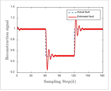
The signals of loss control effectiveness (τ=6): f k₁( )_{and its} estimation: ˆf k1( )

Figure 3

The signals of loss control effectiveness (τ=5): f k2

( )

and its estimation: f kˆ ( )2

0 50 100 150 200 250

-0.2 0 0.2 0.4 0.6 0.8 1 1.2

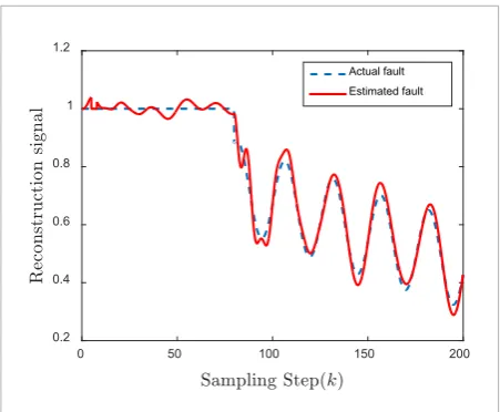
represents the first subsystem is active, while the oth-er subsystem is on running when the switching signal is 1. Simulation results of LOs, which refer to above three component faults, are listed in Figures 2-4. One can see that the proposed LOs can reconstruct the fault signals effectively.

0 30 60 90 120 150 180

0.2 0.4 0.6 0.8 1 1.2 1.4

Actual fault Estimated fault

0 50 100 150 200

0.2 0.4 0.6 0.8 1 1.2 1.4

(8)

Figure 5 shows the fault reconstruction errors. The error tends to converge after small fluctuations with-in a limited time, which proves once agawith-in the

effec-Figure 4

The signals of loss control effectiveness (τ=2) :f k3

( )

and its estimation: ˆf k3( )

0 50 100 150 200

0.2 0.4 0.6 0.8 1 1.2

Table 1

Simulation errors for three component faults

Error Emax Eave Std 1

e 0.4902 0.0031 0.0641

2

e 0.3944 0.0042 0.0706

3

e 0.2248 0.0119 0.0361

Figure 5

The fault reconstruction errors

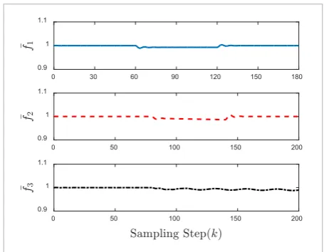
Figure 6

The effect on normal actuator

0 30 60 90 120 150 180

-0.5 0 0.5

0 50 100 150 200

-0.5 0 0.5

0 50 100 150 200

-0.5 0 0.5

tiveness of the proposed scheme. Table 1 presents the simulation errors for the reconstruction of three component faults from a quantitative perspective, while E_max, Eave and Std represent the max value,

average value and standard deviation of the errors. The average error is within the allowable range, while the standard deviation meets the real requirements.

The first actuator is on normal running with f k

( )

=1 for all the time. Figure 6 represents the influence of LOs on the normal actuator, where one can see that the fault reconstruction for a faulty actuator will af-fect another normal one. However, the influence is within the system permissibility.

0 30 60 90 120 150 180

0.9 1 1.1

0 50 100 150 200

0.9 1 1.1

0 50 100 150 200

0.9 1 1.1

1

K plays an important role of “Memory” for the re-constructed fault signal. In general, K1 is a diagonal

matrix with elements close to one. One can deter-mine the value of K1 based on the degree of

fluctua-tion of fault signals. A relatively smaller value of K₁ can help the LOs easily ignore the historical signal and keep track of the fault changes. A simulation experiment to verify the influence of K₁ is estab-lished subject to f k1

( )

. Three values are assigned

to K₁: k₁=0.92I, k₂ =0.95I, k₃=0.98I. Figure 7 presents the simulation results. f k1

( )

has

relative-ly large changes at the sampling point k=60 and

120

(9)

of K1, which can easily ignore the histrorical signal

and keep track of the fault changes. Figure 7 shows that three simulation results all converge to the true fault signal, and the first k₁ value is the best choice with relatively small fluctuations.

Figure 7

Simulation results for f k₁

_{( )}

_{based on different K1}

0 30 60 90 120 150 180

0 0.5

1 1.5

Actual fault k1 k2 k3

In addition, in order to verify the robustness of the proposed component fault diagnosis scheme, an ex-ternal disturbance η_k is added in system (9). There are two actuators in the simulation system. We con-sider two diffenret external noises are as follows:

Figure 8

Simulation results for f k3( ) with external noise

0 50 100 150 200

0.2 0.4 0.6 0.8 1 1.2

(

)

(

)

( )

0.02*sin 3.8* 10

0.01*sin 2.5* ₁₀ +0.01*cos ₈

k

k k

η

 

 

=  

 

 

.

Figure 8 presents the simulation result for f k3

( )

with the external noise. Comparied with the simula-tion result for f k3

( )

without external noise in Figure

4 , there exist some fluctuations for the output of the LOs during the first 100 steps. Then it tends to vary gently. It can also well reconstruct the component faults under the disturbance of external noise.

5. Conclusion

There are relatively few research works for the com-ponent fault diagnosis of switched system. In this pa-per, an active fault detection and estimation scheme based on LOs is investigated against component faults in a class of switched systems. The proposed LOs can guarantee the uniformly ultimately bound-edness of fault reconstruction error with external dis-turbance using switched Lyapunov function and H∞

technique. The design of the LOs is simple and easy to implement, which can deal with different types of fault. In the simulation parts, three kinds of fault re-construction examples have demonstrated the effec-tiveness of the proposed method.

The research of this paper is a supplement to the field of fault diagnosis of switched systems. It can also be extend-ed to other control systems. Future works are as follows:

1 The system involved in this paper is a linear

switched system. However, most switched systems exhibit nonlinear characteristics. It is necessary to consider the effects of nonlinearity.

2 The choice of K1 and τ in the LOs are generally based

on human experience. It should be designed an adap-tive change rule for the parameters in the LOs.

Appendix

There are three parts in the appendix for the proofs of the theorems presented above.

Part A: Proof for Theorem 1: First two lemmas are listed which are useful in the following proof.

(10)

ma-155 Information Technology and Control 2019/1/48

trixP, and two arbitrary matrices M and N with appropriate dimensions, the following inequality holds: ,

2_MPN_≤_γ_MPMT₊_{N PN}T _γ_, ₍₁₇₎

where γ >0.

Lemma 2 [13, 21]: For the fault updating observer es-tablished in (4), the following inequality for fault re-construction error is satisfied

( ) ( )

(

)

(

)

( )(

) (

) ( )

1 1 1

2 2 2 3

T T T

F F F F

T

T T

x i i i i x k k

e k e k e k K K e k

e k K C K C e k F F

ρ τ τ

ρ ρ

≤ − −

+ +   , (18)

where ρ1= + +1 ϑ ϑ1 2, ρ2 = +1 1 +ϑ ϑ1 3 and 2

3 1 1 1 3

ρ = + ϑ + ϑ with ϑ >_i 0, i=1,2,3.

Consider the following Lyapunov function

( )

1 1

1

N T

x i i x

i

k N

T

F i i F

j k i

V k e k k P e k

e j j Q e j

τ

ξ

= −

= − =

 

= _ _

 

 

+ _ _

 

∑

, (19)

where Pi and Qi are the positive defined symmetric

matrices. Then the difference of Lyapunov function is expressed as

( )

(

) ( )

(

)

(

)

(

)

( )

(

)

(

)

(

)

1

1 N 1 1

T

x i i x

i N T

x i i x

i n T

F i i F

i N T

F i i F

i

V k V k V k

e k k P e k

e k k P e k

e k k Q e k

e k k Q e k

ξ

τ ξ τ τ

=

∆ = + −

 

= + _ + _ +

 

 

− _ _

 

 

+ _ _

 

 

− − _ − _ −

 

∑

. (20)

The difference equation (20) above corresponds to any mode of switching rules. As declared in Assump-tion 1, only one subsystem is active each time. So we assume ξ_i

( )

k =1, ξϕ≠_i

( )

k =0, ξj

(

k+ =1 1

)

,

(

1 0

)

j k

ϕ

ξ _≠ + = _,ξ_l

(

k−τ

)

=1, ξ_ϕ≠_l

(

k−τ

)

=0. Then formula (20) can be simplified into

( ) ( ) ( ) ( ) ( ) ( ) ( ) ( ) ( )

( ) ( ) ( ) ( )

( )( ) ( )

( ) ( )

1 1

2

T T

x j x x i x

T T

F i F F l F

T T

x i i i j i i i i x T

T

x i i i j k F T

F l F

T T

F k j k i F

V k e k P e k e k Pe k e k Q e k e k Q e k e k A L C P A L C P e k

e k A L C P U e k e k Q e k

e k U P U Q e k

τ τ

∆ = + + −

+ − − −

 

= _ − − − _

+ −

− − −

 

+ _ + _

. (21)

According to Lemma 1, one can get

( )(

)

( )

( )(

)

(

) ( )

( )

1

2

1

T T

x i i i j k F

T T

x i i i j i i i x

T T

F k j k F

e k A L C P U e k

e k A L C P A L C e k

e k U P U e k

γ γ

− ≤

− −

+

, (22)

where M =e k A LxT

( )(

i− i iC

)

T, P=

(

A Li− i iC

)

T and

( )

k F

N U e k= .

Based on Assumption 2, the formula (21) satisfies the following inequality

( )

( ) (

)(

)

(

)

( )

( ) ( )

(

)

(

)

1

1 i i i T j

T

x x

i i i i

T T

F i F F F

T

F l F

A L C P

V k e k e k

A L C P

e k Q e k e k e k e k Q e k

γ

δ α

τ τ

 

 

⋅ 



+ −

∆ ≤

− −

− +

− − −

 _, ₍₂₃₎

where

(

)

( )

2

(

)

( )

1 max max max

1 1 P uj 1 Ql

α= + γ λ + +δ λ

with δ ≥0.

Applying Lemma 2, the above inequality can be fur-ther expressed as

( )

( ) (

)

(

)

(

)

(

) (

)

( )

(

)

(

)

(

)

1

2 2 2

1 1 1 3

[ 1

] T T

x i i i j i i i

T T

i i i i i x F i F

T T T

F l F k k

V k e k A L C P A L C

P K C K C e k e k Q e k

e k K K Q e k F F

γ

αρ δ

τ αρ τ αρ

∆ ≤ + − −

− + −

+ − − − +  

. (24)

From inequality (7) with Schur complement lemma, one can get

(

)

(

)

(

) (

)

2 2 2 0

T

i i i j i i i i

T

i i i i

A L C P A L C P

K C K C

αρ

− − −

(11)

Let Λ represent the left-hand side of the above inequality, and define λ₁=λ_min

( )

−Λ >0 and

(

)

2 min Qi 0

λ =δλ − > . Together with Assumption 3, one can get

( )

2

( )

2 2

1 x 2 F 3 f

V k λ e k λ e k αρ κ

∆ ≤ − − + . (26)

Thus

( )

3

1 2

max e k_x , e k_F αρ κ_f

λ λ

  ≤

  ₊ . (27)

Hence, the uniform ultimate boundedness of e kx

( )

and e k_F

( )

can be guaranteed.

Part B: Proof for Theorem 2: Consider the following Lyapunov function:

( )

1

( )

2

( )

3

( )

4

( )

V k =V k V k V k V k+ + + , (28) where

( )

1

1 1 2

1 1 3

1 1

4

1 k

N T

x i i x

i

k N

T

x i i x

j k d i

k d k N

T

x i i x

s j i

j k d

k N

T

F i i F

j k i

V k e k k P e k

V k e j j Q e j

V k e s s Q e s

V k e j j R e j

τ

ξ

= −

= − =

− −

= =

= − −

= − =

 

= _ _

 

 

= _ _

 

 

= _ _

 

 

= _ _

 

∑

∑ ∑

∑

. (29)

Then

( )

(

)

(

)

( )

1 Tx 1 j x 1

T

x i x

V k e k P e k

e k Pe k

∆ = + +

− , (30)

( )

(

)

(

)

(

)

(

)

(

)

(

)

2 3 Tx i x

T

x k d x

T

x k d x

T

x k d x

V k V k e k Q e k

e k d Q e k d e k d Q e k d e k d Q e k d

σ

− − −

∆ + ∆ ≤

− − −

, (31)

( )

(

)

(

)

4 TF i F

T

F l F

V k e k R e k e k τ R e k τ

∆ =

− − − , (32)

where σ =

(

d d− +2

)

. Then setting

( )

{

( )

}

min Q min min Qj , j k d k d, 1, ,k d

λ = λ = − − − ⋅⋅⋅ − _{, or}

( )

{

( )

}

min Q min min Q ii ,

λ = λ ∈ℵ , one can get

( )

(

) (

)

2 3

min

T

x i x

T

x k x k

V k V k e k Q e k

Q e k d e k d

σ λ

∆ + ∆ ≤

− − − . (33)

Combining the state estimation error in (11), one can get

(

)

(

)

( )(

)

(

) ( )

(

)

(

)

( )

( )(

)

(

)

( )(

)

( )

( )(

)

(

)

( )

(

)

1 1

2 2 +2 2

2 2

T

x j x

T T

x k di j di x k

T T T T

F k j k F k i j i k T

T

x i i i j di x k T

T

x i i i j k F T T

x i i i j i k

T T

x k di j k F

T T

x k di j i k F

S e k P e k

e k A L C P A L C e k e k d A P A e k d e k U P U e k E P E

e k A L C P A e k d e k A L C P U e k e k A L C P E

e k d A P U e k

e k d A P E e

η η

η

= + +

= − −

+ − −

+ +

+ − −

+ −

−

+ −

+ − +

( )

.

T T

k j i k k U P Eη

(34)

We employ Lemma 1 to simplify the above equation.

For the term 2 T

( )(

)

T

(

)

x i i i j di x k

e k A L C− P A e k d− , one can define M =e k A LTx

( )(

i− i iC

)

T, N=A edi x

(

k d− k

)

,

j

P P= , then

( )(

)

(

)

( )(

)

(

) ( )

(

)

(

)

1

2

1

T T

x i i i j di x k

T T

x k di j di x k

e k A L C P A e k d

e k d A P A e k d γ

γ

− − ≤

− −

+ − −

, (35)

where γ >1 0.

Similarly, one can get

( )(

)

( )

( )(

)

(

) ( )

( )

2

1

T T

x i i i j k F

T T

F k j k F

e k A L C P U e k

e k U PU e k γ

γ

− ≤

− −

+

(12)

( )(

)

( )(

)

(

) ( )

3 3 2 1 T T

x i i i j i k

T T

T T

k i j i k

e k A L C P E

E P E η γ η η γ − − ≤ − + (37)

(

)

( )

(

)

(

)

( )

4 4 2 1 T T

x k di j k F

T T

x k di j di x k

T T

F k j k F

e k d A P U e k e k d A P A e k d

e k U PU e k

γ γ − ≤ − − + (38)

( )

5 5 2 1

T T T T

F k j i k k i j i k

T T

F k j k F

e k U P E E P E

e k U P U e k

η γ η η

γ

≤

+ , (39)

where γ γ γ γ γ >1 2, , 3, ,4 5 0.

Based on Assumption 2, we can get

( )(

)(

)

(

) ( )

(

)

(

)

( )

(

)

1 2 3

4 1 2 ma 4 x 2 3 5 5 1 1 1

1 1 1

1 1 1 2 T T

x i i i

j i i i x

T T

x k di j di x k

T

F j F

T T

k i j i k

T T

x k di j i k

e k A L C

S

P A L C e k

e k d A P A e k d

e k u P e k

E P E e k d A P E

γ γ γ γ γ γ γ γ η _γ γ η η ⋅ +  ₊       _{+ +} ₊ ₋    ≤  −      + − _ + _ − + + + + + + + −       . (40) Thus ( ) ( ) ( )( ) ( ) ( ) ( ) ( ) ( ) ( ) ( ) ( ) ( ) ( ) ( ) ( )

1 2 3

4 1 3 min 5 1 1 1 1 1 2 T i i i T

x x

j i i i i i

T di j di T

x k x k

T T T

k i j i k F i F

T T

F F F l F

T T

x k di j i k

A L C V k e k e k

P A L C Q P A P A

e k d e k d Q

E P E e k R e k e k e k e k R e k

e k d A P E

γ γ γ σ γ γ λ η _γ γ η δ α τ τ η  _{+ +} ₊ ₋    ∆ ≤ ⋅ − + −    _ ₊ ₊ _ _⋅  _ _  + − _ _ − −       + _ + + _ − + − − − + − , (41)

where

( )

( ) ( )

4

2

max max max

2 5

1 1 1

1 u P_j 1 R_i

α= +_ _γ + _γ + _γ _ λ + +δ λ .

Using Lemma 2, we obtain

( ) ( ) ( ) ( ) ( ) ( ) ( ) ( )

(

)

( ) ( ) ( ) ( ) ( ) ( ) ( ) 1

2 2 2

1 1 1 3

2 min

3

2

T

i i i j i i i T

x i i x

T i i i i

T T

F l F

T T T

F i F k i j i k

T T

x k di j di x k

T T T

x k di j i k k k

A L C P A L C V k e k Q P e k

K C K C e k K K R e k

e k R e k E P E

e k d A P A Q e k d e k d A P E F F

ζ σ αρ τ αρ τ δ ζ η η ζ λ η αρ  ₋ _⋅ ₋      ∆ ≤ + −   +    + − − − − +   + − _ − _ − + − +   , (42)

where ζ₁= + +1 γ₁ γ₂+γ₃, ₂ ₄

1

1 1

ζ = + _γ +γ and

3

3 5

1 1

1

ζ = + _γ + _γ .

In order to make the proposed LOs robust to external disturbance, consider the following H∞ performance

index

( ) ( )

2 0

K

T T

y y k k

k

J e k e k γ η η

=

 

=

∑

_ − __, (43)

where K is an arbitrary positive integer. Under zero-initial conditions, one has

( ) ( )

( )

( ) ( )

( )

2 0 2 0 K T T

y y k k

k K

T T

y y k k

k

J e k e k V k V K e k e k V k

γ η η γ η η = =   = _ − + ∆ _−   ≤ _ − + ∆ _

∑

. (44)

It is noted that

( ) ( )

( )

(

)

(

)

(

)

(

)

2 1 3 3 2

T T T

y y k k x x

T T

F F k k

T T x k

x k k

k

e k e k V k e k e k

e k e k F F

e k d e k d

γ η η τ τ αρ η η − + ∆ ≤ Ξ + − Ξ − +  −    +_ − _Ξ       . (45)

Based on Theorem 2 together with Schur complement lemma, one can get Ξ <1 0, Ξ <2 0, Ξ <3 0. Thus

( ) ( )

2

3

0 0

K K

T T T

y y k k k k

k k

e k e k γ η η αρ F F

= =

 − ≤

 

∑

  _. ₍₄₆₎

Thus, the uniform ultimate boundedness of system state estimation error and fault reconstruction error are guaranteed and output estimation error satisfies

3

( )

y f

(13)

Part C: Proof for Theorem 3: Here we give the proof that LMI (12) is equivalent to the formula (15). Simi-larly, LMI (13) can be transformed into the inequality (16).

Assume that (15) is feasible. Then T 0

i i j

G G+ −P >

which means that G_i is nonsingular. For strictly pos-itive matrix Pj, one can get

(

)

T 1

(

)

₀

j i j j i

P G₋ P− P G₋ _≥ _. ₍₄₇₎

Thus

T T T

i j i i i j

G P G G G≥ + −P _. (48)

Then (15) can be transformed into

1 1

2

1

0 0

* 0

0

* * 0

* * * 0

* * * *

T T

i j i i i i i T

i i i i i i

T i i i

G P G G A Y C I

G PG M C G

I C

I

G Q G

ζ

αρ σ

−

₋ ₋ 

 

 ₋ 

 

<

 − 

 ₋ 

 

 ₋ 

 

. ₍₄₉₎

Then, pre multiplying inequality (47) by

{

T, , , , T

}

i i

diag G− I I I G− _{and post multiplying by}

{

1_{, , , ,} 1

}

i i

diag G I I I G− − _{, one can obtain (12). So the}

proof is finished and the parameters of LOs are

calcu-lated by T

i i i

L G Y₌ − _and

2i iT i

K ₌G M− _.

Acknowledgement

This work was supported by the National Natural Sci-ence Foundation of China (No. 61806208, 61502498) and Fundamental Research Funds for the Central Universities (No. 3122017001, 3122017011).

References

1. Bao, L. P., Fei, S. M., Yue, L. Exponential Stability of Linear Distributed Parameter Switched Systems with Time-Delay. Journal of Systems Science and Com-plexity, 2014, 27(2), 263-275. https://doi.org/10.1007/ s11424-014-3070-4

2. Benzaouia, A., Ouladsine, M., Naamane, A., Ananou, B. Fault Detection for Uncertain Delayed Switching Dis-crete-Time Systems. International Journal of Innova-tive Computing, Information and Control, 2012, 8(12), 8049-8062.

3. Blanke, M., Kinnaert, M., Lunze, J., Staroswiecki, M. Diagnosis and Fault-Tolerant Control. Springer, Berlin, 2006.

4. Branicky, M. S. Multiple Lyapunov Functions and Other Analysis Tools for Switched and Hybrid Systems. IEEE Transactions on Automatic Control, 1998, 43(4), 475-482. https://doi.org/10.1109/9.664150

5. Chen, W., Saif, M. An Iterative Learning Observer for Fault Detection and Accommodation in Nonlinear Time-Delay Systems. International Journal of Robust and Nonlinear Control, 2006, 16(1), 1-19. https://doi. org/10.1002/rnc.1033

6. Chiang, M. L., Hsieh, H. C. A New Approach to the Fault Detection Problem for Mobile P2P Network. Infor-mation Technology and Control, 2012, 41(2), 151-161. http://dx.doi.org/10.5755/ j01.itc.41.2.913

7. Daafouz, J., Riedinger, P., Iung, C. C. Stability Anal-ysis and Control Synthesis for Switched Systems: A Switched Lyapunov Function Approach. IEEE Trans-actions on Automatic Control, 2002, 47(11), 1883-1887. https://doi.org/10.1109/TAC.2002.804474

8. Du, D. S., Bin, J., Shi, P., Karimi, H. R. Fault Detection for Continuous-time Switched Systems Under Asynchro-nous Switching. International Journal of Robust and Nonlinear Control, 2014, 24(11), 1694-1706. https://doi. org/10.1002/rnc. 2961

9. Hakem, A., Pekpe, K. M., Cocquempot, V. A Parame-ter-Free Method for Sensor Fault Detection and Isola-tion in Bilinear Systems. Proceedings of 2012 UKACC International Conference on Control, Cardiff, UK, Sep-tember 3-5, 2012, 437-442. https://doi.org/10.1109/ CONTROL. 2012.6334670

10. He, D., Xi, C., Lu, A. Fault Detection for Switched T-S Fuzzy Systems in Finite Frequency Domain. Ad-vances in Difference Equations, 2016, 62. https://doi. org/10.1186/s13662-016-0785-7

11. Hespanha, J. P., Morse, A. S. Stability of Switched Sys-tems with Average Dwell-Time. Proceedings of 38th IEEE Conference on Decision and Control, Phoenix, Arizona, USA, December 7-10, 1999, 2655-2660. https:// doi.org/10.1109/CDC.1999.831330