Analysis of Five Typical Localization Algorithms for Wireless Sensor Networks

http://dx.doi.org/10.4236/wsn.2015.74004

Analysis of Five Typical Localization

Algorithms for Wireless Sensor Networks

Shelei Li, Xueyong Ding, Tingting Yang

Polytechnical School, Sanya College, Sanya, China Email: [email protected]

Received 30 March 2015; accepted 29 April 2015; published 30 April 2015

Copyright © 2015 by authors and Scientific Research Publishing Inc.

This work is licensed under the Creative Commons Attribution International License (CC BY).

http://creativecommons.org/licenses/by/4.0/

Abstract

In this paper, the self-localization problem is studied. It is one of the key technologies in wireless sensor networks (WSNs). And five localization algorithms: Centroid algorithm, Amorphous algo-rithm, DV-hop algoalgo-rithm, APIT algorithm and Bounding Box algorithm are discussed. Simulation of those five localization algorithms is done by MATLAB. The simulation results show that the positioning error of Amorphous algorithm is the minimum. Considering economy and localization accuracy, the Amorphous algorithm can achieve the best localization performance under certain conditions.

Keywords

Wireless Sensor Networks (WSNs), Localization Algorithm, Centroid, Amorphous, DV-Hop, APIT, Bounding Box

1. Introduction

gorithm can realize node localization without distance and angle information, only according to information such as network connectivity, classic algorithms include: centroid, DV-Hop (distance vector-hop), Amorphous, and APIT algorithm. To compare with non-ranging based localization algorithm based on distance measurement for the static characteristic of most sensor network application, the former is curbed in both cost and node size, while the latter does not need additional hardware, there is an advantage in cost and power consumption. On the other hand, the former performance is strongly influenced by environmental factors, while the latter performs well in this respect, and positioning accuracy can meet the requirements of most sensor network applications. In comprehensive view, the latter is more suitable for the characteristics of WSN large-scale network. As a result, most scholars of recent research focus on the Range-free localization algorithm [3].

This paper has analyzed the five classical localization algorithms: Centroid algorithm, Amorphous algorithm, DV-hop algorithm, APIT algorithm and Bounding Box algorithm. And through the comparison among the simu-lation results of five kinds of algorithm performance, and the study of the influence on the localization perfor- mance by anchor node proportion and communication radius, it can provide reference for selecting localization algorithm and configuring parameters [3].

2. Algorithm Introductions

The problem of node localization in wireless sensor networks is to ascertain the location of unknown node according to some localization mechanisms and based on known node. Localization mechanism embodies in localization algorithm. The centroid localization algorithm, Amorphous, DV-hop, APIT and Bounding Box algo-rithm are introduced.

2.1. Centroid Localization Algorithm

Centroid algorithm is put forward by outdoor positioning algorithm of network connectivity in the University of Southern California. The core of the algorithm is that the anchor nodes broadcast a beacon signal to the network every once in a while. The signal itself and location information contained in “received from different when the unknown node anchor node beacon signal exceeds a preset threshold or received after a certain period of time, the node will determine its position for the anchor nodes of polygon centroid”, “literature of centroid algorithm is improved, the density of the proposed adaptive method, the best plans in areas of low anchor node density in-crease of anchor nodes, in order to improve the positioning accuracy”. Fully advantages of the algorithm are based on network connectivity, without coordination between the unknown node and anchor node. The imple-mentation is relatively simple, where shortcoming is positioning accuracy which is not high. A disadvantage of the centroid localization algorithm is that the localization accuracy depends on the density of the anchor node excessively.

2.2. Amorphous Localization Algorithm

Radhika Nagpal has proposed [4] Amorphous algorithm, unlike DV-Hop, it assumes that the average network connectivity of local is known and uses Equation (1) to compute network average hop distance. Among them, r is the communication radius, nlocal is the average network connectivity. The average distance of each hop esti-mated distance multiplied with minimum hop count is calculated to be positioning of nodes, and anchor nodes also need to work out at least three distances, using maximum likelihood estimation to estimate its position or three sided measurements.

2

1 _{ar cos 1}

π

1

HopeSize 1 e e d

nlocal

t t t nlocal

r t

 

−  − − 

−  

−

 

= _ + − _



∫

In essence, the Amorphous algorithm is an enhanced version of DV-Hop algorithm, the gradient correction method and the distance of each hop algorithm calculation, and the introduction of a number of anchor nodes es-timate refinement. The algorithm needs to predict the average connectivity of network and need higher node densities.

2.3. DV-Hop Localization Algorithm

basic principle is to use inter node hop distance to replace the actual distance between nodes.

(

) (

)

HopSize

i j i j

i j i

j i j

x x y y

h ≠

≠

− + −

=

∑

∑

(xi, yi) and (xj, yj) are the coordinates of anchor node i and j, respectively. hj is the jump section number between anchor node i and j (i ≠ j), we can calculate the coordinates of the nodes to be located. The DV-hop al-gorithm is simple, less communication overhead, computation amount is less, the cost is low; but to achieve good positioning accuracy, it needs to decorate the large number of anchor nodes.

2.4. APIT Localization Algorithm [7]

In this section, we describe our novel area-based Range-free localization scheme, which is called APIT. APIT requires a heterogeneous network of sensing devices where a small percentage of these devices (percentages vary depending on network and node density) are equipped with high-powered transmitters and location infor-mation obtained via GPS.

The first step of APIT algorithmic is to determine a plurality of triangular region that contains unknown node, the intersection of these triangular areas is a polygon; then to determine the smaller area including unknown node and calculating the position of the centroid of the polygon, that is, the position of unknown node.

The APIT algorithm can be broken down into four steps: 1) gather information: information of the anchor node near the unknown node, such as the position, identification number, signal strength degree; 2) APIT testing: testing whether the unknown node is internal of the triangle that combined with different anchor nodes; 3) cal-culate overlapping areas: calcal-culate the overlapping area of the all triangles that contain unknown nodes; 4) computing unknown node position: calculate the centroid of the overlapping area and the position of the un-known node. These steps are performed at individual nodes in a purely distributed fashion. Before providing a detailed description of each of these steps, we first present the basic pseudo code for our algorithm.

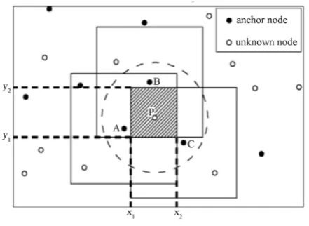
2.5. Bounding Box Algorithm

Semic et al. proposed [8] Bounding Box algorithm.This algorithm uses discrete communication model, and uses a square as communication area, which take r as communication radius and 2r as side length, as shown in

Figure 1.

P is unknown node inFigure 1. Considering P as the center, within the area of r radius, there are A, B and C anchor nodes. To make these squares which take point of A, B, C. as the center respectively and 2r as side leng. then take the centroid of rectangular region of three squares’ intersections as the estimated location of node P. If the P as the center, within the area of r radius, there are k as anchor nodes, the rectangular region centroid of k

squares’ intersection can be the position of the unknown node. The size and position of intersection region can be obtained by Equation (3).

1

2

1

2

max ;

min ;

max ;

min ;

i

i

i

i

y y r

y y r

x x r

x x r

− + − +

(3)

that (xi, yi) is the coordinates of the ith anchor nodes, i=1, 2,k.

3. Simulation and Analysis of Algorithm

To place 200 nodes in an area of 800 m * 800 m randomly, 40 nodes there into are anchor nodes, and the com-munication radius is 200 m. Each time postions of simulation node are generated randomly.Figure 2 is a ran-dom simulation result. It can be obtained from nodes distribution that the average network connectivity is 29.65, the average number of network neighbor anchor nodes is 5.76. By calling the five positioning algorithm proce-dures, positioning error and positioning in the node distribution coverage were obtained, in which the position-ing error of Centroid was 0.28498, the coverage rate of positionposition-ing was 100%; the positionposition-ing error of Amorph- ous was 0.21156, the coverage rate of positioning was 100%; the positioning error of DV-hop was 0.30731, the coverage rate of positioning was 100%; the positioning error of APIT was 0.31168, the coverage rate of posi-tioning was 90%; the posiposi-tioning error of Bounding Box was 0.29328, the coverage rate of posiposi-tioning was 100%. As inFigure 2, red * represents anchor node, blue O represents an unknown node, black O represents an unknown node that con’t be located, blue ― connects the estimates location and the true location, so as to represent localization error.

Due to the random time simulation results cannot explain the problem, 100 times simulation was done under each of the different conditions, and calculated the average localization error to research five algorithms’ per-formance.

In Figure 3 the x-coordinate is the proportion of anchor nodes number to total nodes number, the Y-coordi- nate is the average location error. Figure 3 shows the relation between anchor nodes proportion and localization error of centroid, Amorphous, DV-hop, APT and Bounding Box algorithm, while placing 200 nodes in an areas of m * 800 m. It can be seen from Figure 3 with the increasing of the proportion of anchor node, the average localization error of five algorithms of node showed a trend of decline. The down trend of Bounding Box algo-rithm is the most obvious, because the increase of anchor nodes proportion inevitably leads to the increase of anchor nodes number in each unknown node’s communication radius, and leads to the increase of the number of squares with side length of 2 times the communication radius and taking those anchor nodes as center, then the intersection region of those squares become smaller, so the estimated location of the unknown node becomes more accurate, and the localization coverage rate becomes higher. In the two kinds of algorithms: DV-hop and Amorphous, the main localization error comes from the calculation process of the average distance of each hop, so the decreased trend of localization error is relatively slow while the anchor node proportion increases. The Amorphous algorithm can always achieve fine localization accuracy in different anchor node proportion, taking into account economic factors, the localization performance is fine while the anchor node proportion is 15%.

4. Conclusion

Simulation experiments were carried out to compare the performance of five algorithms and we studied the per-formance change of five algorithms with anchor ratio and communication radius. The simulation results show that the localization error of Amorphous algorithm is minimum. Considering the economic benefits and posi-tioning accuracy, the best localization performance of Amorphous algorithm was achieved when anchor ratio was 20% and communication radius was 200 m in the condition of distributing 200 nodes randomly in 800 m * 800 m square area. The next step will focus on the positioning precision and how to reduce the power consump-tion of nodes and prolong the network lifetime.

Acknowledgements

(a) (b)

(c) (d)

(e) (f) 0 100 200 300 400 500 600 700 800

0 100 200 300 400 500 600 700 800

Node distributeon diagram

0 100 200 300 400 500 600 700 800 0 100 200 300 400 500 600 700 800

Neighbor relationship diagram

0 100 200 300 400 500 600 700 800 0 100 200 300 400 500 600 700 800

Localization error diagram

0 100 200 300 400 500 600 700 800 0 100 200 300 400 500 600 700 800

Localization error diagram

0 100 200 300 400 500 600 700 800 -100 0 100 200 300 400 500 600 700 800

Localization error diagram

0 100 200 300 400 500 600 700 800 0 100 200 300 400 500 600 700 800

(g)

Figure 2. A random simulateion result. (a) Node distributeon diagram. (b) Neighbor relationship diagram. (c) Localization error diagram of Centroid algorithm. (d) Amorphous Localization algorithm. (e) DV-hop Localization algorithm. (f) APIT Localization algorithm. (g) Bounding Localization Box algorithm.

Figure 3. Localization error curve with the change of anchor radio.

This work was supported by the project “the Project Supported by the Scientific Research Fund of the Provincial Natural Science Foundation of Hainan”, the grant number is 614252

Conflict of Interests

The authors declare that there is no conflict of interests regarding the publication of this article.

References

[1] Callaway, E.H. (2004) Wireless Sensor Networks: Architectures and Protocols. CRC Press, Boca Raton, 1-40.

[2] Priyantha, N.B., Balakrishnam, H., Demaine and Teller, S. (2003) Anchor-Free Distributed Localization in Sensor Networks. Proceedings of the 1st International Conference on Embedded Networked Sensor System, Los Angeles, 5-7 November 2003, 340-341.

[3] Zhang, Z., Hong, S. and Ren, T.J. (2010) Discussion on Localization Algorithm of Wireless Sensor Networks. Journal of Guizhou University (Natural Science), 27, 99-102.

[4] Nagpal, R., Shrobe, H. and Bachrach, J. (2003) Organizing a Global Coordinate System from Local Information on an 0 100 200 300 400 500 600 700 800

0 100 200 300 400 500 600 700 800

Localization error diagram

0.05 0.1 0.15 0.2 0.25 0.3

0.2 0.25 0.3 0.35 0.4 0.45 0.5 0.55

Ad Hoc Sensor Network. Information Processing in Sensor Networks Lecture Notes in Computer Science, 2634, 333-348.

[5] Nicolescu, D. and Nath, B. (2001) Ad-Hoc positioning systems (APS). Proceedings of the 2001 IEEE Global Tele-communications Conference, San Antonio, 25-29 November 2001, 2926-2931.

http://dx.doi.org/10.1109/GLOCOM.2001.965964

[6] Dai, Y., Wang, J.P. and Zhang, C.W. (2010) Research and Improvement of Localization Algorithms for Wireless Sen-sor Network. Journal of Transduction Technology, 23, 567-570.

[7] He, T., Huang, D.C., Blum, B.M., Stanjovic, J.A. and Abdelzaher, T. (2003) Range-Free Localization Schemes for Large Scale Sensor Networks.Proceedings of the 9th Annual International Conference on Mobile Computing and Networking (MobiCom’03), San Diego, 14-19 September 2003, 81-95.