www.earth-syst-sci-data.net/6/69/2014/ doi:10.5194/essd-6-69-2014
©Author(s) 2014. CC Attribution 3.0 License. Open
Access
Science
Data
An update to the Surface Ocean CO
2
Atlas (SOCAT
version 2)
D. C. E. Bakker1, B. Pfeil2,3, K. Smith4,5, S. Hankin4, A. Olsen2,3,6, S. R. Alin4, C. Cosca4, S. Harasawa7, A. Kozyr8, Y. Nojiri7, K. M. O’Brien4,5, U. Schuster9,*, M. Telszewski10, B. Tilbrook11,12, C. Wada7, J. Akl11, L. Barbero13, N. R. Bates14, J. Boutin15, Y. Bozec16,17, W.-J. Cai18, R. D. Castle19, F. P. Chavez20,
L. Chen21,22, M. Chierici23,24, K. Currie25, H. J. W. de Baar26, W. Evans4,27, R. A. Feely4, A. Fransson28,
Z. Gao21, B. Hales29, N. J. Hardman-Mountford30, M. Hoppema31, W.-J. Huang18, C. W. Hunt32,
B. Huss19, T. Ichikawa33, T. Johannessen2,3,6, E. M. Jones31, S. D. Jones34, S. Jutterström35, V. Kitidis36,
A. Körtzinger37, P. Landschützer1, S. K. Lauvset2,3, N. Lefèvre38,39, A. B. Manke4, J. T. Mathis4,
L. Merlivat15, N. Metzl15, A. Murata40, T. Newberger41, A. M. Omar6,3,2, T. Ono33, G.-H. Park42,
K. Paterson11, D. Pierrot13, A. F. Ríos43, C. L. Sabine4, S. Saito44, J. Salisbury32, V. V. S. S. Sarma45, R. Schlitzer31, R. Sieger31, I. Skjelvan6,2,3, T. Steinhoff37, K. F. Sullivan13, H. Sun21, A. J. Sutton4,5,
T. Suzuki46, C. Sweeney41, T. Takahashi47, J. Tjiputra6,3, N. Tsurushima48, S. M. A. C. van Heuven49,
D. Vandemark32, P. Vlahos50, D. W. R. Wallace51, R. Wanninkhof19, and A. J. Watson9,*
1Centre for Ocean and Atmospheric Sciences, School of Environmental Sciences, University of East Anglia,
Norwich Research Park, Norwich, UK
2Geophysical Institute, University of Bergen, Bergen, Norway
3Bjerknes Centre for Climate Research, Bergen, Norway
4Pacific Marine Environmental Laboratory, National Oceanic and Atmospheric Administration, Seattle,
Washington, USA
5Joint Institute for the Study of the Atmosphere and Ocean, University of Washington, Seattle, Washington,
USA
6Uni Climate, Uni Research, Bergen, Norway
7National Institute for Environmental Studies, Tsukuba, Japan
8Carbon Dioxide Information Analysis Center, Oak Ridge National Laboratory, Oak Ridge, Tennessee, USA
9College of Life and Environmental Sciences, University of Exeter, Exeter, UK
10International Ocean Carbon Coordination Project, Institute of Oceanology of the Polish Academy of
Sciences, Sopot, Poland
11CSIRO Marine and Atmospheric Research, Hobart, Australia
12Antarctic Climate and Ecosystems Cooperative Research Centre, Hobart, Australia
13Cooperative Institute for Marine and Atmospheric Studies, Rosenstiel School for Marine and Atmospheric
Science, University of Miami, Miami, Florida, USA
14Bermuda Institute of Ocean Sciences, Ferry Reach, Bermuda
15Sorbonne Universités (UPMC, Univ Paris 06), CNRS, IRD, MNHN, LOCEAN Laboratory, Paris, France
16CNRS, UMR 7144, Equipe Chimie Marine, Station Biologique de Roscoff, Roscoff, France
17Sorbonne Universités, UPMC Université Paris 06, UMR7144, Adaptation et Diversité en Milieu Marin, SBR,
Roscoff, France
18School of Marine Science and Policy, University of Delaware, Newark, Delaware, USA
19Atlantic Oceanographic and Meteorological Laboratory, National Oceanic and Atmospheric Administration,
Miami, Florida, USA
20Monterey Bay Aquarium Research Institute, Moss Landing, California, USA
21Key Laboratory of Global Change and Marine-Atmospheric Chemistry, Third Institute of Oceanography,
State Oceanic Administration, Xiamen, P. R. China
23Institute of Marine Research, Tromsø, Norway
24Department of Chemistry and Molecular Biology, University of Gothenburg, Gothenburg, Sweden
25National Institute of Water and Atmospheric Research, Dunedin, New Zealand
26Royal Netherlands Institute for Sea Research, Texel, the Netherlands
27Ocean Acidification Research Center, University of Alaska Fairbanks, Fairbanks, Alaska, USA
28Norwegian Polar Institute, Fram Centre, Tromsø, Norway
29College of Earth, Ocean and Atmospheric Sciences, Oregon State University, Corvallis, Oregon, USA
30CSIRO Marine and Atmospheric Research, Floreat, WA, Australia
31Alfred Wegener Institute Helmholtz Centre for Polar and Marine Research, Bremerhaven, Germany
32Ocean Process Analysis Laboratory, University of New Hampshire, Durham, New Hampshire, USA
33National Research Institute for Fisheries Science, Fisheries Research Agency, Yokohama, Japan
34Tyndall Centre for Climate Change Research, University of East Anglia, Norwich Research Park, Norwich, UK
35IVL Swedish Environmental Research Institute, Gothenburg, Sweden
36Plymouth Marine Laboratory, Plymouth, UK
37GEOMAR, Helmholtz Centre for Ocean Research, Kiel, Germany
38IRD, Sorbonne Universités (UPMC, Univ Paris 06), CNRS, MNHN, LOCEAN Laboratory, Paris, France
39LaboMar, Universidade Federal do Ceará, Fortaleza-Ceará, Brazil
40Japan Agency for Marine-Earth Science and Technology, Yokosuda, Japan
41Cooperative Institute for Research in Environmental Sciences, University of Colorado, Boulder, Colorado, USA
42East Sea Research Institute, Korea Institute of Ocean Science and Technology, Uljin, Korea 43Instituto de Investigaciones Marinas de Vigo, Consejo Superior de Investigaciones Científicas, Vigo, Spain
44Marine Division, Global Environment and Marine Department, Japan Meteorological Agency, Tokyo, Japan
45National Institute of Oceanography, Regional Centre, Visakhapatnam, India
46Marine Information Research Center, Japan Hydrographic Association, Tokyo, Japan
47Lamont Doherty Earth Observatory, Columbia University, Palisades, New York, USA
48National Institute of Advanced Industrial Science and Technology, Tsukuba, Japan
49Centre for Isotope Research, University of Groningen, Groningen, the Netherlands
50Department of Marine Sciences, University of Connecticut, Groton, Connecticut, USA
51Department of Oceanography, Dalhousie University, Halifax, Canada
∗formerly at: School of Environmental Sciences, University of East Anglia, Norwich Research Park, Norwich, UK
Correspondence to: D. C. E. Bakker ([email protected])
Received: 25 June 2013 – Published in Earth Syst. Sci. Data Discuss.: 16 August 2013 Revised: 12 January 2014 – Accepted: 24 January 2014 – Published:
Abstract. The Surface Ocean CO2 Atlas (SOCAT), an
ac-tivity of the international marine carbon research
commu-nity, provides access to synthesis and gridded f CO2
(fu-gacity of carbon dioxide) products for the surface oceans. Version 2 of SOCAT is an update of the previous release (version 1) with more data (increased from 6.3 million to
10.1 million surface water f CO2 values) and extended data
coverage (from 1968–2007 to 1968–2011). The quality con-trol criteria, while identical in both versions, have been ap-plied more strictly in version 2 than in version 1. The SOCAT website (http://www.socat.info/) has links to quality control comments, metadata, individual data set files, and synthe-sis and gridded data products. Interactive online tools allow visitors to explore the richness of the data. Applications of SOCAT include process studies, quantification of the ocean carbon sink and its spatial, seasonal, year-to-year and longer-term variation, as well as initialisation or validation of ocean carbon models and coupled climate-carbon models.
Data coverage
Repository-References: Individual data set files and
synthesis product: doi:10.1594/PANGAEA.811776
Gridded products:
doi:10.3334/CDIAC/OTG.SOCAT_V2_GRID
Available at: http://www.socat.info/ Coverage: 79◦S to 90◦N; 180◦W to 180◦E Location Name: Global Oceans and Coastal Seas
Date/Time Start: 16 November 1968
Date/Time End: 26 December 2011
1 Introduction
Human activity is releasing large quantities of the
green-house gas carbon dioxide (CO2) into the atmosphere. As a
result, the atmospheric CO2mole fraction has increased from
280µmol mol−1 in pre-industrial times (Jansen et al., 2007)
The rapid, ongoing change in the atmospheric composition by greenhouse gas emissions has been predicted to increase
global mean temperature by 1.5◦C to 5.0◦C by the end of
the century (Peters et al., 2013). Such warming would be ac-companied by sea level rise, increased storm frequency, melt-ing of ice caps and sea ice, changes in precipitation patterns and ocean acidification (Solomon et al., 2007), to name only the most prominent examples. Already many changes in the Earth’s climate are apparent, such as the decline in Arctic sea ice extent (Stroeve et al., 2007), and warming in Alaska, near the Antarctic Peninsula (Vaughan et al., 2003; Mulvaney et al., 2012) and of the upper ocean (Levitus et al., 2005).
The oceans absorb a substantial part of the CO2
emis-sions by human activity, thereby mitigating climate change. From pre-industrial times to 1994 the oceans have taken up 118±19 Pg C from the atmosphere (Sabine et al., 2004). This
is equivalent to roughly 50 % of CO2 emissions from
fos-sil fuel burning and cement production or 30 % of the
to-tal anthropogenic emissions, if CO2 emissions from land
use change are included. Recent estimates indicate that the oceans are a contemporary sink for roughly 27 % of the
an-nual CO2 emissions by fossil fuel combustion, cement
pro-duction and land use change (Le Quéré et al., 2013). Uncer-tainty in the land use change emissions leads to a large error estimate for the proportion of the anthropogenic emissions taken up by the oceans.
There is uncertainty on how much CO2the oceans will
ab-sorb in a warming climate of the future (e.g. Jones et al., 2013). Considerable year-to-year, decadal and longer-term
variation of CO2 uptake is apparent in the North Atlantic
Ocean (Corbière et al., 2007; Schuster and Watson, 2007; Thomas et al., 2008; Schuster et al., 2009; McKinley et al., 2011), the North Sea (Thomas et al., 2007), the North Pacific Ocean (Takamura et al., 2010), the equatorial Pacific Ocean (Feely et al., 2002, 2006; Ishii et al., 2004, 2009; Park et al., 2006, 2012) and the Southern Ocean (Le Quéré et al., 2007; Metzl, 2009), with large differences between ocean regions (Le Quéré et al., 2010; Lenton et al., 2012).
Measurements of CO2in the surface oceans (generally
ex-pressed as the mole fraction of CO2 (xCO2), partial
pres-sure (pCO2), or fugacity ( f CO2)) enable estimation of CO2
air–sea fluxes and their variability. The fugacity can be mea-sured underway on the surface water supply of ships. This method is used on a variety of ships, including ships of
op-portunity on commercial routes. The number of CO2
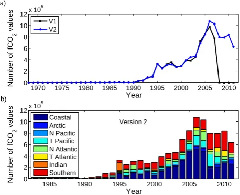
mea-surements has greatly increased over the past four decades (Fig. 1) (Sabine et al., 2010). Data collection started in the late 1960s and 1970s, increased in the 1980s and intensi-fied from the 1990s onwards. Roughly four times more data have been collected during the 2000s than in the 1990s. The growth in data collection has partly resulted from large in-ternational research programmes, for example JGOFS (Joint Global Ocean Flux Study) and WOCE (World Ocean Cir-culation Experiment), and regional funding initiatives. The development of autonomous instrumentation for the
contin-1970 1975 1980 1985 1990 1995 2000 2005 2010 0
2 4 6 8 10 12x 10
5
Year
Number of fCO
2
values
a)
V1 V2
1985 1990 1995 2000 2005 2010 0
2 4 6 8 10 12x 10
5
Year
Number of fCO
2
values Version 2
b)
Coastal Arctic N Pacific T Pacific N Atlantic T Atlantic Indian Southern
Figure 1.(a) The number of surface water f CO2values per year in
SOCAT versions 1 and 2 and (b) per region per year in version 2. The SOCAT operationally defined region names are the Coastal Seas, the Arctic Ocean, the North Pacific Ocean, the Tropical Pa-cific Ocean, the North Atlantic Ocean, the Tropical Atlantic Ocean, the Indian Ocean and the Southern Ocean (Fig. 5, Table 5). These data points originate from data sets with flags of A, B, C or D and have a WOCE flag of 2. The subsequent figures only show f CO2
values with these characteristics.
uous measurement of surface water f CO2(e.g. Körtzinger et
al., 1996; Cooper et al., 1998; Pierrot et al., 2009), the inter-comparison of such instrumentation at sea (Körtzinger et al., 1996, 2000) and its installation on ships of opportunity (e.g. Cooper et al., 1998; Lüger et al., 2004; Schuster and Watson, 2007; Watson et al., 2009; Takamura et al., 2010; Lefèvre et al., 2013) and on moorings and drifters (e.g. Hood et al., 1999; Emerson et al., 2011) have played an important role in the increase in data collection.
Quantification of global and regional, annual mean ocean
CO2 uptake requires observations of surface water f CO2
with adequate spatial and temporal coverage (Sweeney et al., 2000; Lenton et al., 2006). Studies of year-to-year, decadal
and longer-term trends in air–sea CO2 uptake necessitate
consistent, multi-decade data records of surface ocean f CO2
(e.g. Schuster and Watson, 2007; Park et al., 2012). Statisti-cal techniques and modelling have been developed to infer
basin-wide distributions of surface water f CO2 from
lim-ited observations, for example a diffusion–advection based interpolation scheme (Takahashi et al., 1997, 2009), (multi-ple) linear regression (e.g. Boutin et al., 1999; Sarma et al., 2006), neural network approaches (e.g. Lefèvre et al., 2005) and a diagnostic ocean mixed layer model (Rödenbeck et al., 2013).
Uniform procedures for the collection, reporting,
process-ing and archivprocess-ing of CO2 data, as well as public release of
2008-2011 a)
1968-2011
80°N
40°N
0°
40°S
80°S b)
80°N
40°N
0°
40°S
80°S
100°E 160°W 60°W 40°E
100°E 160°W 60°W 40°E
Surface water fCO2 (µatm)
240 280 320 340 350 360 370 380 390 400 440
Figure 2.The global distribution of surface water f CO2values in
SOCAT version 2: (a) for 1968 to 2011 and (b) for 2008 to 2011.
and co-workers have constructed an impressive series of
sur-face ocean CO2 climatologies, the most recent one for the
climatological year 2000 (Takahashi et al., 2009), and now
provide annual updates to their global surface ocean pCO2
data set (Takahashi et al., 2013). The Surface Ocean CO2
At-las (SOCAT) (Bakker et al., 2012; Pfeil et al., 2013; Sabine et al., 2013) complements this work. The SOCAT and Taka-hashi data sets benefit from standardisation and intercompar-ison of measurement and reporting protocols, as well as dis-cussions between data providers and quality controllers on reporting standards and data quality (Dickson et al., 2007; IOCCP, 2008; SOCAT, 2011; Wanninkhof et al., 2013a). Both data sets contribute towards more rapid availability of ocean carbon data for synthesis products and policy-related assessments.
SOCAT is an international activity of ocean carbon scien-tists. It aims to create, make publicly available and archive the following (IOCCP, 2007):
– A 2nd level quality-controlled, global surface ocean
f CO2 data set following internationally agreed-upon
procedures and regional review;
– A gridded data product of mean monthly surface water
f CO2 on a 1◦latitude by 1◦ longitude grid with
mini-mal temporal or spatial interpolation using the 2nd level quality-controlled, global surface ocean f CO2data set.
The first SOCAT release was made public as versions 1.4 and 1.5, here jointly referred to as version 1, in Septem-ber 2011 (Bakker et al., 2012). SOCAT version 1 contains 6.3 million surface f CO2data points from 1851 data sets in
the global oceans and coastal seas between 1968 and 2007 (Fig. 1, Table 1) (Pfeil et al., 2013; Sabine et al., 2013). Ver-sion 2 is presented here.
2 SOCAT version 2
2.1 An update of version 1
Version 2 is an update of version 1 with 60 % more data and 4 years extra data coverage. SOCAT version 2 contains 10.1 million surface f CO2values from 2660 data sets for the
global oceans and coastal seas between November 1968 and December 2011 (Figs. 1 and 2). Version 2 was made pub-lic on 4 June 2013 at the 9th International Carbon Dioxide Conference in Beijing, China (SOCAT, 2013b).
SOCAT data products provide surface water f CO2values
at sea surface temperature ( f CO2rec, with “rec” indicating
recommended f CO2), which have been (re-)calculated from
the original CO2 values reported by the data provider,
fol-lowing a strict calculation protocol. Sea surface temperature refers to the temperature at the seawater intake, often at about 5 m depth on ships. The procedures for data retrieval, for data entry, for the (re-)calculation of surface water f CO2, for
quality control, and for the creation of data products in ver-sion 2 are analogous to those used in verver-sion 1 (Pfeil et al., 2013; Sabine et al., 2013) and are described in Sects. 2.2, 2.3 and 2.4. The sections also highlight where version 2 differs from version 1 (Table 1).
Version 2 has three data products (Tables 2 and 3):
1. Individual data set files of surface water f CO2in a
uni-form uni-format which have been subject to 2nd level qual-ity control;
2. A synthesis data set of surface water f CO2 for the
global oceans and coastal seas;
3. Global gridded products of surface water f CO2means.
These data products are much the same as those for version 1 (Sect. 2.4) (Pfeil et al., 2013; Sabine et al., 2013). The SO-CAT website (http://www.socat.info/) provides access to the data products together with online visualisation tools, data documentation, quality control comments, meeting reports, publications and a list of contributors (Tables 4, 5 and 6).
2.2 Data assembly and (re-)calculation of fCO2in
version 2 2.2.1 Data origin
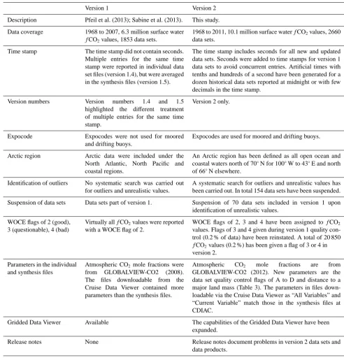
Table 1.Key differences between SOCAT versions 1 (released as versions 1.4 and 1.5) and 2. Further details are in the text.
Version 1 Version 2
Description Pfeil et al. (2013); Sabine et al. (2013). This study.
Data coverage 1968 to 2007, 6.3 million surface water
f CO2values, 1853 data sets.
1968 to 2011, 10.1 million surface water f CO2values, 2660
data sets.
Time stamp The time stamp did not contain seconds.
Multiple entries for the same time stamp were reported in individual data set files (version 1.4), but were averaged in the synthesis files (version 1.5).
The time stamp includes seconds for all new and updated data sets. Seconds were added to time stamps for version 1 data sets to avoid concurrent entries. Artificial times with tenths and hundreds of a second have been generated for a dozen historical data sets reported at midnight or with few decimals in the time stamp.
Version numbers Version numbers 1.4 and 1.5
highlighted the different treatment of multiple entries for the same time stamp.
Version 2 only.
Expocode Expocodes were not used for moored
and drifting buoys.
Expocodes are used for moored and drifting buoys.
Arctic region Arctic data were included under the
North Atlantic, North Pacific and coastal regions.
An Arctic region has been defined as all open ocean and coastal waters north of 70◦
N for 100◦
W to 43◦
E and north of 66◦N elsewhere.
Identification of outliers No systematic search was carried out for outliers and unrealistic values.
A systematic search for outliers and unrealistic values has been carried out. In total 154 data sets have been suspended.
Suspension of data sets Data sets part of version 1. Suspension of 70 data sets included in version 1 upon identification of unrealistic values.
WOCE flags of 2 (good), 3 (questionable), 4 (bad)
Virtually all f CO2values were reported
with a WOCE flag of 2.
WOCE flags of 2, 3 and 4 have been assigned to f CO2
values. Flags of 3 and 4 given during version 1 quality con-trol (0.2 % of data) have been reinstated. A total of 20 850
f CO2values (0.2 %) has been given a flag of 3 or 4 in
version 2.
Parameters in the individual and synthesis files
Atmospheric CO2 mole fractions were
from GLOBALVIEW-CO2 (2008).
The files downloadable from the
Cruise Data Viewer contained more parameters than the synthesis files.
Atmospheric CO2 mole fractions are from
GLOBALVIEW-CO2 (2012). New parameters are the data set quality control flags of A to D and distance to a major land mass (Table 3). The parameters in files down-loadable via the Cruise Data Viewer as “All Variables” and “Current Variable” match those in the synthesis files at CDIAC.
Gridded Data Viewer Available The capabilities of the Gridded Data Viewer have been
expanded.
Release notes None Release notes document problems in version 2 data sets and
data products.
Carbon Dioxide Information Analysis Center (CDIAC),
PANGAEA®, institutions and research projects. Version 2
has an additional 3.8 million surface f CO2 values and
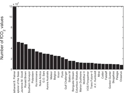
807 data sets relative to version 1, mostly from 2006 to 2011 (Fig. 1, Table 1). Figure 3 shows the number of f CO2values
from the 30 ships, including 1 ship-based time series, with the most intense data collection effort. The data sets in ver-sion 2 originate from 107 different ships, plus 3 ship-based
time series, 13 mooring-based time series and 3 drifters (Ta-ble 7). This study will adopt the term “data set” rather than “cruise” for individual data sets to reflect the presence of mooring and drifter data (0.7 % of f CO2values in version 2).
Table 2.Key characteristics of the three SOCAT data products for surface ocean f CO2values in version 2 (Sect. 2.4). The synthesis product
is available as synthesis files and as subsets of the global synthesis data set. The table lists whether the data products include only f CO2
data with a WOCE flag of 2 (good) or also with flags of 3 (questionable) and 4 (bad). Information on access to metadata and quality control comments is provided. All data products can be accessed via the SOCAT website (http://www.socat.info) and via the links in the table.
Characteristics WOCE
flag
Metadata QC entries
Access and format
Individual data set files
The files contain all original CO2 measurements and f CO2values with a flag of 2, 3 and 4 for data sets with
flags of A, B, C or D. Metadata accompany the files.
2, 3, 4 Yes No Text files at
Pangaea1
Synthesis data set
Synthesis files consist of data sets with flags of A, B, C and D and contain f CO2values with a flag of 2. The
global synthesis data set is available as global2,3and re-gional files2.
2 only No No Zip text files2
and in Ocean Data View format3
Subset of synthesis data set (i)
Subset of the synthesis data set containing f CO2values
with a flag of 2. Selection of “Include SOCAT invalids” gives access to f CO2values with a flag of 2, 3 and 4.
2 as default; 2, 3, 4 upon request
No No Text files via
Cruise Data Viewer4
Subset of synthesis data set (ii)
Subset of the synthesis data set containing original CO2
measurements and f CO2values with a flag of 2, 3 and
4. Metadata and quality control entries are available.
2, 3, 4 Yes Yes Text files
via Table of Cruises4
Gridded files Gridded means of f CO2 values on a 1◦×1◦ grid with
minimal interpolation. Means are per year, monthly per year, monthly per decade and per climatological month from 1970 to 2011. A monthly 0.25◦×
0.25◦
data set is available for coastal regions.
2 only No No NetCDF files5,
in Ocean Data View format3,
and via Gridded Data Viewer6
1doi:10.1594/PANGAEA.811776,2http://cdiac.ornl.gov/ftp/oceans/SOCATv2/,
3http://odv.awi.de/en/data/ocean/socat_fCO2_data,4http://ferret.pmel.noaa.gov/SOCAT2_Cruise_Viewer/, 5http://cdiac.ornl.gov/ftp/oceans/SOCATv2/SOCATv2_Gridded_Dat/, doi:10.3334/CDIAC/OTG.SOCAT_V2_GRID, 6http://ferret.pmel.noaa.gov/SOCAT_gridded_viewer/
As in version 1 (Sect. 3.1 in Pfeil et al., 2013), most surface
water CO2values have been measured by equilibration of a
headspace with seawater and subsequent analysis of the CO2
content of the headspace. Historical measurements generally used gas chromatographic analysis, while more recent mea-surements are based on infrared detection. SOCAT versions 1 and 2 include a small number of historical, discrete surface
water f CO2measurements. SOCAT products do not include
f CO2calculated from other carbon parameters, such as pH,
alkalinity or dissolved inorganic carbon. A small percentage
of the f CO2 values (0.2 % in version 2) is from
measure-ments by a spectrophotometric method using a pH-sensitive dye (Table 7) (e.g. Hood et al., 1999).
2.2.2 Data entry
The data were assembled in a uniform file format, as in ver-sion 1 (Sect. 3.2 in Pfeil et al., 2013). Key differences in data entry between versions 1 and 2 relate to the time stamp, ver-sion numbering and an expocode for moorings and drifters, as described in Sect. 2.2.3.
Primary quality control was carried out at this stage. Pri-mary quality control included identification of basic prob-lems in the data, for example unrealistic positions, times and orders of magnitude. Additional basic problems were identi-fied during secondary quality control (Sect. 2.3).
2.2.3 Key differences with version 1 in data entry Time stamp and version numbering: the time stamp for SO-CAT version 1 products did not contain seconds (Table 1) (Pfeil et al., 2013). In some cases this resulted in multiple entries for a given time stamp. Such multiple entries were averaged in the synthesis files (version 1.5), but not in the individual data set files (version 1.4). Two version numbers (version 1.4 and 1.5) highlight the different treatment of mul-tiple entries for the same time stamp in the version 1 data products (Table 1).
Table 3.Content of the individual data set files (IF) and the synthesis files in SOCAT version 2. The global synthesis product is available as zip text files at CDIAC (ZIP) and in Ocean Data View (ODV) format. Subsets of the global synthesis data set can be created via the Cruise Data Viewer for All Variables (CDV_AV), Current Variable (CDV_CV) and via the Table of Cruises (CDV_TC). The first column (“Notation”) lists column headers for the parameters in the files.
Notation IF ZIP, CDV_CV ODV CDV_TC Unit Description
CDV_AV
Expocode – X X X X – 12-character expocode
SOCAT_DOI – X X X X – Digital object identifier for the
individual data set and metadata
QC_ID – X 2 –
X – Data set quality control flag with
11 for A, 12 for B, 13 for C and 14 for D
Date/Time X – X – – – yyyy-mm-dd/hh:mm:ss
(ISO8859)
yr – X – X X Year Year (UTC)1
mon – X – X X Month Month (UTC)1
day – X – X X Day Day (UTC)1
hh – X – X X Hour Hour (UTC)1
mm – X – X X Minute Minute (UTC)1
ss – X – X X Seconds Seconds (may include decimals)1
Time – – 2 – – Hour Hours since 1970
Day of Year – – 2 – – Day of Year Day of Year (UTC) with
1 January 00:00 as 1.0.
Longitude X X X X X ◦
E Longitude (0 to 360)1
Latitude X X X X X ◦N,◦S Latitude (−90 to 90)1
Sample_depth/Depth water X X 2 X X m Water sampling depth1,3
Sal X X 2
X X – Salinity on Practical
Salinity Scale1
Temp/SST X X 2
X X ◦
C Sea surface temperature1
Tequ X X 2
X X ◦
C Equilibrator chamber
temperature1
PPPP X X 2
X X hPa Atmospheric pressure1
Pequ X X 2 X X hPa Equilibrator chamber pressure1
WOA_SSS/Sal interp X X 2 X X – Salinity from WOA (2005)4
NCEP_SLP/PPPP interp X X 2
X X hPa NCEP Atmospheric pressure5
ETOPO2_depth/Bathy depth interp X X 2 X X m ETOPO2 Bathymetry6
Distance/d2l X X 2 – X km Distance to major land mass
GVCO2/xCO2air_interp X X 2
X X µmol mol−1 Atmospheric xCO2from
GLOBALVIEW-CO2 (2012)
xCO2water_equ_dry X – – – X µmol mol−1 xCO
2(water) at equilibrator
temperature (dry air)1
f CO2water_SST_wet X – – – X µatm f CO2(water) at sea surface
temperature (air at 100 %
humidity)1
pCO2water_SST_wet X – – – X µatm pCO2(water) at sea surface
temperature (air at 100 %
humidity)1
xCO2water_SST_dry X – – – X µmol mol−1 xCO
2(water) at sea surface
temperature (dry air)1
f CO2water_equ_wet X – – – X µatm f CO2(water) at equilibrator
temperature (air at 100 %
humidity)1
pCO2water_equ_wet X – – – X µatm pCO2(water) at equilibrator
temperature (air at 100 %
humidity)1
f CO2rec/f CO2water_SST_wet X X 2 X X µatm Recommended f CO2calculated
following the SOCAT protocol
f CO2rec_src/Algorithm X X 2
X X – Algorithm for calculating
f CO2rec (0: not generated; algo-rithm 1–14 in Table 8)
f CO2rec_flag/Flag X X 2
-X – WOCE flag for f CO2rec (2:
good, 3: questionable, 4: bad)7
1Data reported by the data originator. 2Available upon selection of parameter.
3If the intake depth has not been reported by the data originator, an intake depth of 5 m has been assumed.
4Sea surface salinity on the Practical Salinity Scale interpolated from the World Ocean Atlas (WOA) 2005 (Antonov et al., 2006), available at:
http://www.nodc.noaa.gov/OC5/WOA05/pr_woa05.html (last access: 1 May 2013).
5Atmospheric pressure interpolated from the NCEP/NCAR (National Centers for Environmental Prediction/National Center for Atmospheric Research) 40-Year Reanalysis Project on a
6-hourly, global, 2.5◦latitude by 2.5◦longitude grid (Kalnay et al., 1996), available at: http://www.esrl.noaa.gov/psd/data/gridded/data.ncep.reanalysis.surface.html (last access: 1 May
2013).
6Bathymetry interpolated from ETOPO2 (2006) 2-minute Gridded Global Relief Data, available at: http://www.ngdc.noaa.gov/mgg/global/etopo2.html (last access: 1 May 2013). 7Individual data set files contain all f CO
Table 4.Activities and key participants in SOCAT versions 2 and 3 to date. Regional group leads are in Table 5.
Activity Key Participants
Global group for coordination
Bakker (chair), Hankin, Kozyr, Metzl, Olsen, Pfeil, Pierrot, Telszewski
Data retrieval, data entry, (re-)calculation of
f CO2
Pfeil, Olsen
Quality control Alin, Bakker, Barbero, Castle, Cosca, Evans, Hales, Harasawa, Hoppema, Huang, Hunt, Huss, Park, Paterson, Pierrot, Schuster, Skjelvan, Steinhoff, Suzuki, Tilbrook, Van Heuven, Vlahos, Wada, Wanninkhof
Live Access Server
Hankin, O’Brien, Smith
Individual data set files, synthesis products and gridded products
Pfeil, Smith, Manke, Hankin
Ocean Data View Schlitzer
Matlab files Pierrot, Landschützer
SOCAT website Pfeil
Data archiving and online access
Pfeil, Sieger, Kozyr, Smith, Manke, Hankin
Meetings Alin, Bakker, Hales, Hankin, Nojiri,
Telszewski
Alternative sensors (version 3)
Wanninkhof, Steinhoff, Bakker, Bates, Boutin, Olsen, Sutton
Automation (versions 3 to 4)
Hankin, S. Jones, Kozyr, O’Brien, Pfeil, Smith, Bakker, Olsen, Schweitzer
data sets, seconds were added artificially to the time stamp to avoid the problem of multiple entries. The next version of SOCAT will include seconds, as reported by the data contrib-utor, for all data sets.
The CO2 measurements for a dozen historical data sets
are listed at midnight or their time stamp in fractional days contains insufficient decimals for retrieving minutes and sec-onds. Artificial seconds, in some cases including tenths or hundreds of a second, were generated for these valuable data,
such that they can remain in SOCAT version 2. Every effort
will be made to retrieve a more adequate time stamp for these data sets for future versions. Unlike version 1, which has ver-sion 1.4 and 1.5 data products, verver-sion 2 data products have a single version number (Table 1).
Expocode for moorings and drifters: SOCAT uses twelve character expocodes (Swift, 2008) as stable and unique data set identifiers. For example, 49P120101218 indicates a cruise on the Japanese (49) ship of opportunity Pyxis (P1) with the first day of the cruise on 18 December 2010. In contrast to version 1, expocodes have been assigned for moorings and drifters in version 2, by registering a “vessel code” at Inter-national Council for the Exploration of the Sea (ICES) in collaboration with the National Oceanographic Data Cen-ter (NODC) and the British Oceanographic Data Centre (BODC) (Table 1).
2.2.4 (Re-)calculation of recommended fCO2
Surface water f CO2 values at sea surface temperature (or
intake temperature), also known as recommended f CO2
( f CO2rec), have been recalculated, analogous to version 1
(Sect. 3.3 in Pfeil et al., 2013). A single set of equations and a strict order of preference for the CO2 input parameter has
been used (Table 8) (Pfeil et al., 2013). Six different CO2
parameters were reported in the original data files, notably xCO2, pCO2and f CO2, either at the equilibration
tempera-ture (Tequ) or at the sea surface temperatempera-ture (SST).
The (re-)calculation procedure of f CO2has the following
philosophy (Pfeil et al., 2013):
1. Whenever possible, (re-)calculate f CO2;
2. The favourite starting point for the calculations is xCO2,
next pCO2, followed by f CO2;
3. Minimise the amount of external data required for the calculations.
Table 8 lists surface water CO2parameters and ancillary
pa-rameters used for calculation of recommended f CO2in
ver-sion 2 in order of preference with algorithm 1 as the favourite (analogous to Table 4 in Pfeil et al., 2013). The algorithm is provided in the output files (Table 3). Equations recom-mended by Dickson et al. (2007) have been used for the con-version of the dry CO2 mole fraction to pCO2, for the
cal-culation of the water vapour pressure and for the conversion of pCO2 to f CO2, similar to version 1 (Sect. 3.3 of Pfeil
et al., 2013). As in version 1, the correction of Takahashi et al. (1993) has been applied for temperature change between the seawater intake and the site of equilibration:
f CO2SST = f CO2equTexp 0.0423(SST - Tequ). (1)
Climatological values of salinity and atmospheric pressure from reanalysis have been used in the calculation of recom-mended f CO2(Table 8), if the data contributor did not report
Table 5.Regions and regional group leads in SOCAT version 2 (Fig. 5).
Region Definition Lead(s)
Coastal Seas Less than 400 km from land; between 30◦S and 70◦N Alin, Cai, Hales
for 100◦
W to 43◦
E; between 30◦
S and 66◦
N elsewhere Arctic Ocean North of 70◦
N for 100◦
W to 43◦
E; north of 66◦
N Mathis
elsewhere, including coastal waters North Atlantic 30◦
N to 70◦
N Schuster
Tropical Atlantic 30◦
N to 30◦
S Lefèvre
North Pacific 30◦
N to 66◦
N Nojiri
Tropical Pacific 30◦N to 30◦S Cosca
Indian Ocean North of 30◦
S Sarma
Southern Ocean South of 30◦
S, including coastal waters Tilbrook, Metzl
Table 6.Meetings for SOCAT versions 2 and 3 to date.
Timing Meeting description Location Reference
09/2011 Public release of version 1. Session on future SOCAT.
UNESCO, Paris, France (SOCAT, 2011)
05/2012 Automation planning meeting NOAA-PMEL, Seattle, USA (SOCAT, 2012a)
07/2012 SOCAT progress meeting Epochal Centre, Tsukuba, Japan
(SOCAT, 2012b)
10/2012 Coastal and Arctic SOCAT quality control workshop
NOAA-PMEL, Seattle, USA (IOCCP, 2012)
06/2013 SOCAT side event at the 9th International Carbon Dioxide Conference. Public release of version 2.
Beijing International Convention Center, Beijing, China
(SOCAT, 2013b)
2.3 Secondary quality control in version 2
2.3.1 Secondary quality control criteria
Criteria for 2nd level quality control have been defined in a series of workshops (IOCCP, 2008, 2009, 2010; Pfeil et al., 2013). Second level quality control consists of assigning a quality control flag to each data set and a WOCE flag to individual surface water f CO2values. The criteria for quality
control are identical in versions 1 (Sect. 4.1 in Pfeil et al., 2013) and 2.
Only data sets with a quality control flag of A, B, C and D are included in SOCAT version 1 and 2 data products (Table 9) (Pfeil et al., 2013). The data set quality control flags (formerly known as “cruise flags”) in versions 1 and 2 have been developed for automated shipboard measurement
of surface water f CO2, mainly by infrared detection and
frequent at sea standardisation using calibration gases with
a range of CO2 concentrations (IOCCP, 2008; Pfeil et al.,
2013). Much weight is put on whether approved methods or standard operating procedures (SOP) (AOML, 2002; Dick-son et al., 2007; Pierrot et al., 2009) were followed by mak-ing this a prerequisite for flags of A and B. Citmak-ing Pfeil et al. (2013):
“Seven SOP criteria need to be fulfilled for a cruise (or data set) flag of A or B in SOCAT:
1. The data are based on xCO2analysis, not f CO2
calcu-lated from other carbon parameters, such as pH, alka-linity or dissolved inorganic carbon;
2. Continuous CO2 measurements have been made, not
discrete CO2measurements;
3. The detection is based on an equilibrator system and is measured by infrared analysis or gas chromatography;
4. The calibration has included at least 2 non-zero gas standards, traceable to World Meteorological Organiza-tion (WMO) standards;
5. The equilibrator temperature has been measured to within 0.05◦C accuracy;
6. The intake seawater temperature has been measured to within 0.05◦C accuracy;
7. The equilibrator pressure has been measured to within 0.5 hPa accuracy.”
The f CO2 values from data sets with flags of A and B are
0 2 4 6 8 10 12x 10
5
Number of fCO
2
values
Nathaniel B. Palmer Explorer of the Seas Laurence M. Gould
Ronald Brown
Southern Surveyor
Polarstern
Ka imimoana Nuka Arctica
G.O. Sars
Aurora Australis
Meteor Belgica Knorr Pyxis
Gulf Challenger
Station M
Benguela Stream Columbus Waikato Marion Dusfresne
McArthur II
VOS Finnpartner Trans Future
−
5
A.V. Humboldt
Mirai
Colibri Falstaff
Gordon Gunter
Skogafoss
Pelagia
Oceanus
Figure 3.The number of surface water f CO2values obtained on
the 30 ships, including 1 ship-based time series, hosting the most intense data collection effort in SOCAT version 2.
also needs to be met for flags of C and D, similar to version 1 (Sect. 4.1 in Pfeil et al., 2013). Complete metadata documen-tation is required for data set quality control flags of A, B and C. Comparison to other data is carried out, if possible. The overall quality of the data needs to be deemed acceptable for flags of A, B, C and D (Table 9) (Pfeil et al., 2013).
The Southern and Indian Ocean groups (Table 5) have ap-plied three additional quality control criteria for the tempera-ture change between the seawater intake and the equilibrator in versions 1 and 2 (IOCCP, 2010), citing Pfeil et al. (2013):
– “Warming should be less than 3◦C;
– Warming rate should be less than 1◦C h−1, unless a
rapid temperature front is apparent;
– Warming outliers should be less than 0.3◦C, compared
to background data.”
In addition:
– Cooling between the seawater intake and the
equilibra-tor is unlikely in high-latitude oceans for an indoor mea-surement system;
– Zero or constant temperature change may indicate
ab-sence of SST values.
The above five guidelines have been applied widely in ver-sion 2 for open ocean data away from sea ice, as part of a sys-tematic search for unrealistic data and outliers (Sect. 2.3.3). Such a systematic search has not been carried out for ver-sion 1 (Table 1).
These quality control criteria (Table 9) have also been ap-plied for quality control of surface water CO2measurements
from moorings and drifters in versions 1 and 2 (Table 7).
Individual f CO2 values are assigned WOCE flags: 2
(good), 3 (questionable) or 4 (bad) with 2 being the default
Europe USA Asia&Australia
0 5 10 15 20
Number of QC−ers
V1 V2
Figure 4.The number of quality controllers in SOCAT versions 1 and 2 based in Europe, the USA, Asia and Australia, respectively. The figure demonstrates the international character of the quality control effort in SOCAT.
setting (Sect. 4.1.3 in Pfeil et al., 2013). Outliers in parame-ters required for the timing, position and (re-)calculation of f CO2values are given flags of 3 and 4. Thus, flags of 3 and
4 might indicate an erroneous time or position stamp, an un-realistic seawater temperature, strong warming between the seawater intake and the equilibrator or a large pressure diff er-ence between the equilibrator and the atmosphere. Data sets with a large number of flags of 3 and 4 (>50, as a guide line) are suspended, as was also the case for version 1 (Pfeil et al., 2013).
2.3.2 Secondary quality control in practice
Secondary quality control for version 2 has been carried out by 24 marine carbon scientists from eight countries (Fig. 4, Table 4). Quality control in SOCAT is carried out by groups organised according to region. These regions have been op-erationally defined and do not necessarily follow common oceanographic definitions. Regions for version 2 are the Coastal Seas, the North Atlantic, Tropical Atlantic, North Pacific, Tropical Pacific, Indian Ocean and Southern Oceans and a newly defined Arctic region (Fig. 5, Table 5). The Arc-tic region includes both coastal seas and the deep ocean. It encompasses all waters north of 70◦N for 100◦W to 43◦E
(Atlantic sector) and north of 66◦N elsewhere (Table 1)
(Sect. 2.3.3) (SOCAT, 2012b).
Table 7.Drifters and time series in SOCAT version 2 with the location, year(s) of operation, platform type, CO2instrument type, algorithm
used for (re-)calculation of f CO2(Table 8), number of data sets, number of f CO2values with a WOCE flag of 2, and reference.
Drifters and time series Location Year(s) Platform type CO2instrument type Algorithm Number Number Reference
data f CO2
sets values
CARIOCA 75.0◦N 3.0◦W 1996–1997 Drifter Membrane spectrophotometer 6 1 2668 H1999
CARIOCA 0.4◦
S 7.8◦
W 1997 Drifter Membrane spectrophotometer 6 1 1964 B2001
CARIOCA 40.1◦
S 15.8◦
E 2005 Drifter Membrane spectrophotometer 6 1 1451 BM2009
PIRATA_10W_6S 6◦S 10◦W 2006–2007 Mooring Membrane spectrophotometer 6 2 11 820 L2008
Papa_145W_50N 50.1◦N 144.8◦W 2007 Mooring Equilibrator-IR 6 1 4987 J2010
JKEO_147E_38N 37.9◦
N 146.6◦
E 2007 Mooring Equilibrator-IR 6 1 927 J2010
KEO_145E_32N 32.3◦N 144.5◦E 2007–2008 Mooring Equilibrator-IR 6 2 4740 J2010
MOSEAN_158W_23N 22.8◦N 158.1◦W 2004–2007 Mooring Equilibrator-IR 6 5 6034 J2010
WHOTS_158W_23N 22.7◦
N 158.1◦
W 2007 Mooring Equilibrator-IR 6 1 4750 J2010
CRIMP1 21.4◦N 157.8◦W 2005 Mooring Equilibrator-IR 6 1 1993 J2010
TAO_170W_0 0.0◦S 170.0◦W 2005 Mooring Equilibrator-IR 6 1 2577 J2010
TAO_155W_0 0.0◦
W 155.0◦
W 2005 Mooring Equilibrator-IR 6 1 2198 J2010
TAO_140W_0 0.0◦N 139.8◦W 2004–2007 Mooring Equilibrator-IR 6 5 5253 J2010
TAO_125W_0 0.2◦S 124.4◦W 2004–2007 Mooring Equilibrator-IR 6 4 3686 J2010
BTM_64W_32N 31.8◦
N 64.2◦
W 2005–2007 Mooring Equilibrator-IR 6 3 5095 J2010
Stratus_85W_20S 19.7◦
S 85.6◦
W 2006 Mooring Equilibrator-IR 6 1 9466 J2010
Station M 66.0◦N 2.0◦E 2006–2007 Ship Equilibrator-IR 1 19 159 671 WT1993
Station P 50◦
N 145◦
W 1973–1976 Ship Equilibrator-IR 6 12 4158 None
Western Channel Observatory 50.1◦
N 4.3◦
W 2007–2009 Ship Equilibrator-IR 1 1 899 HM2008, K2012
References are: B2001 – Bakker et al. (2001); BM2009 – Boutin and Merlivat (2009); H1999 – Hood et al. (1999); HM2008 – Hardman-Mountford et al. (2008); J2010 – Johengen (2010); K2012 – Kitidis et al. (2012); L2008 – Lefèvre et al. (2008); WT1993 – Wanninkhof and Thoning (1993).
Figure 5.Quality control regions for SOCAT version 2 (Table 5). White shading corresponds to the coastal region. The regions have been defined for operational reasons and do not necessarily reflect common oceanographic definitions.
data set flags between regions and decide on the “agreed” flag for a data set. The data set quality control flag has been added as a parameter in the synthesis files (Tables 1 and 3) (Sects. 2.4.4 and 2.4.7).
Overall data quality and reporting of metadata has im-proved from version 1 to version 2, which we attribute to the SOCAT effort. In version 1, 41 % of the data sets were as-signed a flag of A or B, 22 % obtained a flag of C and, 37 % received a flag of D. Version 2 has a larger proportion of data
sets with flags of A or B (48 %) and smaller proportions of data sets with a flag of C (18 %) and D (33 %).
2.3.3 Key differences with version 1 in secondary quality control
This section identifies key differences in secondary quality control between versions 1 and 2.
Creation of an Arctic regional designation: in version 1 Arctic data were part of the North Pacific and North At-lantic Oceans and the Coastal Region (Sect. 2.2 in Pfeil et al., 2013). Given the importance of Arctic research and the rapid increase in the quantity of Arctic f CO2values, an Arctic
re-gion has been defined for version 2 (Figs. 5 and 6; Table 1) (Sect. 2.3.2) (SOCAT, 2012b).
Identification of unrealistic values: in version 2 a sys-tematic search has been carried out for unrealistic values or patterns in all data relevant for the timing, position or (re-)calculation of f CO2 (Sect. 2.3.1). This activity
consid-ered all the data sets submitted to version 2, including data sets previously included in the version 1 data release. The search applied to the ship’s cruise track, position, time, at-mospheric pressure, equilibrator pressure, salinity, sea sur-face temperature, equilibrator temperature, and temperature change between the seawater intake and the equilibrator. This helped locate problems with data entry, e.g. overlap between data sets, reversal of hours and minutes, reversal of SST and salinity, presence of undefined values (e.g.−999,−99,
Table 8.Surface water CO2parameters used for the calculation of recommended f CO2( f CO2rec) at sea surface temperature in version 2
(after Table 4 in Pfeil et al., 2013). The parameters are listed in order of preference (with algorithm 1 as the favourite). The algorithm is provided in the output files (Table 3). In cases of incomplete data reporting, these ancillary parameters have been used for atmospheric pressure and salinity: NCEP (National Centers for Environmental Prediction) atmospheric pressure (Kalnay et al., 1996) and WOA (World Ocean Atlas) salinity (Antonov et al., 2006) (Sect. 2.2.4).
Algorithm Reported CO2 Unit Data Extra
parameter Percentage (%) variable
1 xCO2water_equi_dry µmol mol−1 66.7 –
2 xCO2water_SST_dry µmol mol−1 4.5 –
3 pCO2water_equi_wet µatm 4.5 –
4 pCO2water_SST_wet µatm 2.6 –
5 f CO2water_equi µatm 0.2 –
6 f CO2water_SST_wet µatm 10.8 –
7 pCO2water_equi_wet1 µatm 0.3 NCEP Pressure
8 pCO2water_SST_wet1 µatm 8.3 NCEP Pressure
9 xCO2water_equi_dry2 µmol mol−1 0.2 WOA Salinity
10 xCO2water_SST_dry2 µmol mol−1 0.7 WOA Salinity
11 xCO2water_equi_dry1 µmol mol−1 0.01 NCEP Pressure
12 xCO2water_SST_dry1 µmol mol−1 1.0 NCEP Pressure
13 xCO2water_equi_dry1,2 µmol mol−1 0.01 NCEP Pressure,
WOA Salinity
14 xCO2water_SST_dry1,2 µmol mol−1 0.1 NCEP Pressure,
WOA Salinity
1Atmospheric pressure was not reported in the original data file. 2Salinity was not reported in the original data file.
the problem, this resulted in suspension of a data set (Ta-ble 10) or assignation of a WOCE flag of 3 (questiona(Ta-ble) or 4 (bad) to individual f CO2values.
In total, 154 data sets have been suspended, of which 70 had previously been included in the version 1 release (Ta-ble 1). Ta(Ta-ble 10 lists grounds for suspension of data sets.
These include absence of CO2 values (14 %), a data entry
problem (10 %), use of a constant atmospheric pressure or salinity in the calculation of f CO2 (45 %), absence of SST
(8 %), and concerns on the quality of f CO2 (3 %),
tempera-ture (14 %), or atmospheric pressure (2 %). In case of a data entry problem, data sets will be re-entered into the SOCAT quality control system for version 3. In other cases, data sets may need revision before resubmission to SOCAT. Finally, six data sets (4 %) made by a spectrophotometric method were suspended, as the data set flags of A to D were not deemed appropriate by the quality controller. In response, a new data set flag of E has been defined for use in version 3 (Sect. 4.2) (Wanninkhof et al., 2013a).
Suspension of 70 data sets included in version 1: 70 data sets previously included in version 1 were suspended from version 2 upon identification of data quality concerns (Ta-bles 1 and 10), as discussed above. Most of these (59) were suspended as a constant atmospheric pressure had been used in the calculation of f CO2. These 59 data sets have since
been revised and resubmitted to SOCAT for version 3. Six data sets were suspended for a data entry problem, while three data sets lacked surface water CO2values. Concerns on
the quality of a temperature or atmospheric pressure reading were grounds for suspension of a further two data sets.
WOCE flags of 3 and 4: WOCE flags of 2 (good), 3 (ques-tionable) and 4 (bad) have been assigned to all f CO2 values
in version 2, including for data sets part of the version 1 re-lease. During version 1 quality control, 0.2 % of the f CO2
values had been assigned a flag of 3 or 4. However, these flags were accidentally reset to a flag of 2 prior to the ver-sion 1 release, such that most f CO2values in version 1 were
reported with a flag of 2. The initial flags of 3 and 4 set during version 1 quality control have been reinstated in version 2. In
version 2, a total of 20 850 f CO2 values (0.2 %) has been
given a flag of 3 or 4.
2.4 Version 2 data policy and data products 2.4.1 Data policy
Users of the SOCAT data products are requested to do the following (SOCAT, 2013a, b):
1. Recognise the contribution of SOCAT data contributors and quality controllers in the form of invitation to co-authorship or citation of relevant scientific articles by data contributors;
Table 9.Criteria for assigning data set quality control flags based on the expected quality of the recommended f CO2values (per Table 6 in
Pfeil et al., 2013). All criteria need to be met for assigning a data set flag. Only data sets with a quality control flag of A, B, C and D are included in version 1 and 2 data products. SOP is Standard Operating Procedures (Dickson et al., 2007); QC is quality control.
Data set flag (ID) Criteria
A (11) 1. Followed approved methods or SOP criteria and
2. Metadata documentation complete and 3. Extended QC was deemed acceptable and
4. A comparison with other data was deemed acceptable.
B (12) 1. Followed approved methods or SOP criteria and
2. Metadata documentation complete and 3. Extended QC was deemed acceptable.
C (13) 1. Did not follow approved methods or SOP criteria but 2. Metadata documentation complete and
3. Extended QC was deemed acceptable (including comparison with other data if possible).
D (14) 1. Did or did not follow approved methods or SOP criteria and 2. Metadata documentation incomplete but
3. Extended QC was deemed acceptable (including comparison with other data if possible).
S (Suspend) 1. Did or did not follow methods or SOP criteria and 2. Metadata documentation complete or incomplete and 3. Extended QC revealed non-acceptable data but 4. Data are being updated.
X (15) (Exclude) The data set duplicates another data set in SOCAT.
N (No flag) No data set flag has yet been given to this data set.
U (Update) The data set has been updated.
No data set flag has yet been given to the revised data.
3. Send references of publications using SOCAT products to [email protected].
2.4.2 SOCAT data products
The SOCAT data products provide access to recommended surface ocean f CO2values in a uniform format for the global
oceans and coastal seas. Three different SOCAT data
prod-ucts are available: individual data set files, synthesis files and gridded files. User-defined subsets of the synthesis files are available via the Cruise Data Viewer. The Gridded Data Viewer facilitates querying of the gridded data products. All data products can be accessed via the SOCAT website (http://www.socat.info/) or via the web-links provided below. Table 2 identifies the key characteristics of the SOCAT data products, while Table 3 lists the contents of downloadable files. The version 2 data products resemble those for ver-sion 1 (Pfeil et al., 2013; Sabine et al., 2013), apart from further standardisation and extra parameters. The data prod-ucts and tools are discussed below, followed by a
descrip-tion of key differences between version 1 and 2 (Table 1)
(Sect. 2.4.7).
2.4.3 Individual data set files
Individual data set files provide surface water f CO2, the
pa-rameters used to (re-)calculate f CO2 and the original CO2
parameter(s) reported by the data contributor for data sets with a flag of A, B, C or D (Table 2). The files include
all surface water f CO2 values with WOCE flags of 2, 3
and 4. Individual data set files are archived at PANGAEA®
(doi:10.1594/PANGAEA.811776). Each data set has a
dig-ital object identifier (doi) (Table 3). Metadata provided by the data contributor accompany the data set files. As in ver-sion 1, the individual data set and synthesis files include the climatological values of salinity and atmospheric pressure from reanalysis. The files also contain values for the water depth, the distance to a major land mass and the atmospheric
CO2 mole fraction interpolated from GLOBALVIEW-CO2
(2012). Via PANGAEA®, version 2 is made available to the
Table 10.Grounds for suspension of data sets from SOCAT version 2. A distinction is made between data sets previously included in version 1 and new data sets in version 2. Abbreviations are SST for sea surface temperature, Tequ for equilibrator temperature and dT for the difference between the equilibrator temperature and the sea surface temperature.
Ground for suspension Number data Number data Percentage of
sets version 1 sets version 2 total (%)
Overlap with other data set 0 1 1
Data entry problem (incomplete data set, time, position, SST, salinity)
6 9 10
Constant atmospheric pressure in calculation of f CO2rec
59 5 42
Constant salinity (0 or−999) in calculation of f CO2rec
0 5 3
No xCO2, pCO2or f CO2reported 3 19 14
No SST reported 0 13 8
Concerns on quality of f CO2rec 0 4 3
Concerns on quality of SST, Tequ or dT 1 20 14
Concerns on quality of atmospheric pressure
1 2 2
No appropriate sensor flag 0 6 4
Total 70 84 100
2.4.4 Global synthesis product
The global synthesis data set consists of individual data sets
with flags of A, B, C and D and contains f CO2 values
with a WOCE flag of 2 (Table 2). The synthesis files do not contain the original CO2 values (Table 3). Each line in
the files lists the doi-number of the corresponding individual data set file at PANGAEA®(Sect. 2.4.3). The synthesis data set is available as global and regional files for the SOCAT regions (Fig. 5). The regional files only contain data from within that region, so that data from most cruises are split between several regional files. The global and regional files are publicly available as compressed zip text files via CDIAC (http://cdiac.ornl.gov/ftp/oceans/SOCATv2/). Matlab code is available for reading these synthesis files. The global syn-thesis product is also available in Ocean Data View format (http://odv.awi.de/en/data/ocean/socat_fCO2_data).
2.4.5 Subsetting the global synthesis product
The Cruise Data Viewer (http://ferret.pmel.noaa.gov/
SOCAT2_Cruise_Viewer/), an interactive tool on the Live
Access Server, enables searching and subsetting the global synthesis data set by year, month, day, region, parameter, expocode, cruise name, vessel, and data set quality control flag. One may define search limits, for example salinity below 32. The user can create property-property plots and download data. The default setting is access to f CO2values
with a WOCE flag of 2 (Table 2). However, the user can include data with flags of 3 (questionable) and 4 (bad) by selecting “Include SOCAT invalids”. Figures 2 and 7 have been made with the Cruise Data Viewer.
The Table of Cruises, available via the pull-down menu “Tables” on the Cruise Data Viewer, enables the user to find metadata and read quality control comments for specific data sets (Table 2). Files downloadable via the Table of Cruises
contain f CO2values with WOCE flags of 2, 3 and 4 and the
original CO2data (Table 3).
2.4.6 Gridded products
Sabine et al. (2013) detail the gridding of the f CO2values on
a 1◦latitude by 1◦longitude grid with a higher 0.25◦latitude by 0.25◦ longitude resolution product for the coastal seas in version 1. The procedures for gridding the data are identical in versions 1 and 2.
Several gridded products of surface ocean f CO2
means with minimal interpolation are available
(doi:10.3334/CDIAC/OTG.SOCAT_V2_GRID). Surface
water f CO2 values with a flag of 2 have been put on a 1◦
latitude by 1◦longitude grid in four ways: per year, monthly per year, monthly per decade, and per climatological month
from 1970 to 2011 (Table 2). A higher resolution of 0.25◦
latitude by 0.25◦ longitude is available as monthly means
per year for the coastal region (Fig. 5).
Gridded f CO2 values are reported as unweighted means
and as cruise-weighted (or data set-weighted) means (Sabine et al., 2013). In an unweighted mean all the recommended f CO2 values in a grid cell have been given equal weight in
calculating the mean. In a cruise-weighted mean, first
aver-ages of the recommended f CO2 values per cruise (or data
set) have been calculated within a grid cell, before averages of the cruise means have been determined. Grid cells
with-out f CO2 values are empty. No correction has been made
Coastal Arctic N Pacific T Pacific N Atlantic T Atlantic Indian Southern 0
1 2 3 4 5 6 7
Density (count/100 km
2 )
V1 V2
Figure 6.The density of surface water f CO2 values for each
re-gion in SOCAT versions 1 and 2. Rere-gions are the Coastal Seas, the Arctic Ocean, the North Pacific Ocean, the Tropical Pacific Ocean, the North Atlantic Ocean, the Tropical Atlantic Ocean, the Indian Ocean and the Southern Ocean (Fig. 5, Table 5). In version 1, Arctic data were included in the North Pacific, North Atlantic and Coastal Regions.
something users of the monthly climatological and decadal gridded products should keep in mind. Furthermore, the grid-ded products may have a temporal bias in grid cells with un-even temporal data coverage. For example, an annual gridded product may have a strong seasonal bias, if only summertime
f CO2values are available.
Gridded f CO2 products can be accessed as NetCDF files
from CDIAC (http://cdiac.ornl.gov/ftp/oceans/SOCATv2/
SOCATv2_Gridded_Dat/), in Ocean Data View format (http:
//odv.awi.de/en/data/ocean/socat_fCO2_data) and via the
Gridded Data Viewer (http://ferret.pmel.noaa.gov/SOCAT_
gridded_viewer/) (Table 2). Matlab code is available for read-ing the NetCDF files.
The capabilities of the Gridded Data Viewer have been
expanded in version 2. The number of different years is a
new variable in the monthly climatological gridded data set. The Gridded Data Viewer now shows the 400 km continental margin mask at 1 min resolution used for defining the Coastal Region (Table 5) and the distance to the nearest major land mass from 0 to 1000 km at 20 min resolution. The Gridded Data Viewer has an option for animation of gridded prod-ucts. The interface has a new comparison capability for up to four gridded data sets. This enables the user to visualise, for example, gridded data products in SOCAT versions 1 and 2 in a multiple-plot view.
2.4.7 Key differences with version 1 in the data products This section identifies key differences between the data prod-ucts for versions 1 and 2.
Parameters in the individual and synthesis data set files: the data set quality control flags of A to D have been added as numerical values 11 to 14 to the synthesis files in ver-sion 2 (Tables 1 and 3). The distance to a major land mass is
a new parameter in the files. Atmospheric CO2 mole
frac-tions from the 2012 GLOBALVIEW-CO2 are reported in version 2 output files; this represents an update from the 2008 GLOBALVIEW-CO2 values which were reported for
a)
80°N
40°N
0°
40°S
80°S b)
80°N
40°N
0°
40°S
80°S
100°E 160°W 60°W 40°E
100°E 160°W 60°W 40°E
Surface water fCO2 (µatm)
240 280 320 340 350 360 370 380 390 400 440
JFM 2000s
JAS 2000s
Figure 7.Seasonal distribution of surface water f CO2 values for
2000 to 2009 in SOCAT version 2 for (a) January to March and (b) July to September.
version 1. The number of parameters in the downloadable files available via the Cruise Data Viewer as “All Variables” and “Current Variable” has been strongly reduced to match those in the synthesis files at CDIAC (Tables 1 and 3).
Gridded Data Viewer: the number of different years has been added as a variable to the monthly climatological grid-ded data set (Sect. 2.4.6). Data sets for the 400 km continen-tal margin mask and the distance to the nearest major land mass are now available. The visualisation tools of the Grid-ded Data Viewer have been expanGrid-ded.
Release notes: release notes document issues identified with individual data sets or data products in version 2. The notes are available on the CDIAC (http://cdiac.ornl.gov/ ftp/oceans/SOCATv2/) and SOCAT (http://www.socat.info/ access.html) websites (Table 1).
3 Spatial and temporal data coverage
SOCAT version 2 includes surface ocean f CO2values
Figure 8. The number of (a) months of the year and (b) total months with surface water f CO2 values in each 1◦ latitude by 1◦
longitude grid cell from 1970 to 2011 in SOCAT version 2. Fig-ure 8a updates a similar figFig-ure for version 1 in Sabine et al. (2013, Fig. 5).
For example, version 2 has a total of 40 data sets in the Arctic Ocean, of which 10 data sets were collected in 2011 alone. Data coverage remains sparse in large parts of the Southern Hemisphere oceans (Fig. 2).
On average 3.4 surface water f CO2values have been
col-lected per 100 km2 between 1968 and 2011 in the global
oceans and coastal seas. Data density ranges widely from 0.8 f CO2 values per 100 km2 in the Indian Ocean to 6.7 values
per 100 km2in the North Atlantic Ocean (Fig. 6). Data
den-sity in the Southern Ocean appears somewhat high with 2.6 values per 100 km2 relative to the North Pacific, the
Tropi-cal Pacific and the TropiTropi-cal Atlantic Oceans. However, the Southern Ocean includes coastal waters with higher than av-erage data density (Fig. 5), while the other three open ocean regions do not. Five of the ten most “productive” ships in terms of data collection are active south of 30◦S, notably the Nathaniel B. Palmer, the Laurence M. Gould, the Southern Surveyor, the Polarstern and the Aurora Australis (Fig. 3).
The seasonal distribution of surface water f CO2 values
is shown in Fig. 7 for the period 2000 to 2009. The maps demonstrate the near absence of wintertime data in the high-latitude regions. The Ross Sea (Southern Ocean) has about 20 months of observations spanning five months from aus-tral spring to autumn (Fig. 8).
The installation of automated f CO2 systems on ships of
opportunity and Antarctic supply ships has greatly improved the data availability along shipping routes and including for coastal seas near major ports (Fig. 9). For example, between 2000 and 2009 more than 40 individual ship visits have been
made to the 1◦ latitude by 1◦ longitude grid boxes in the
a) b)
c) d)
0 8 16 24 32 40
100°W 90°W 80°W 70°W 60°W 20°W 10°W 0° 10°E 50°N
40°N
30°N
20°N
10°N
60°N
50°N
40°N
224 0 8 16 24 32 40 157
0 8 16 24 32 40 185 131
50°S
60°S
70°S
0 8 16 24 32 40
130°E 140°E 150°E 160°E 76°W 68°W 60°W 52°W 50°N
40°N
30°N
20°N
Figure 9.Number of data sets (colour bar on top of subplots) with surface water f CO2 measurements per 1◦ latitude by 1◦ longitude
grid cell for 2000 to 2009 for (a) the northwest Atlantic Ocean and the Caribbean Sea, (b) the northeast Atlantic Ocean and European shelf seas, (c) the northwest Pacific Ocean and (d) Drake Passage in the Southern Ocean. The presence of repeated f CO2 observations
made on ships of opportunity and research supply ships is clearly visible in coastal seas and the open ocean.
Florida Straits, the English Channel, offthe coast of Japan and near the Antarctic Peninsula.
The numbers of unique months and total months with f CO2 values per 1◦ latitude by 1◦ longitude grid cell shed
light on data collection activities for 1970 to 2011 (Fig. 8). High data density along shipping routes highlights the
re-peated f CO2 observations. For example, numerous grid
boxes east of Japan have observations in all months of the year for about 50 months in total, reflecting an intense CO2
observational effort over a large number of years. This ongo-ing data collection effort is critical for the quantification of the variability and trends in CO2air–sea exchange.
4 Future plans
4.1 Progress towards version 3
Surface water CO2 values and accompanying metadata can