www.geosci-model-dev.net/8/2355/2015/ doi:10.5194/gmd-8-2355-2015
© Author(s) 2015. CC Attribution 3.0 License.
Three-dimensional visualization of ensemble weather forecasts –
Part 2: Forecasting warm conveyor belt situations for aircraft-based
field campaigns
M. Rautenhaus1, C. M. Grams2, A. Schäfler3, and R. Westermann1
1Computer Graphics & Visualization Group, Technische Universität München, Garching, Germany 2Institute for Atmospheric and Climate Science, ETH Zürich, Zurich, Switzerland
3Deutsches Zentrum für Luft- und Raumfahrt, Institut für Physik der Atmosphäre, Oberpfaffenhofen, Germany Correspondence to: M. Rautenhaus ([email protected])
Received: 4 February 2015 – Published in Geosci. Model Dev. Discuss.: 27 February 2015 Revised: 23 June 2015 – Accepted: 7 July 2015 – Published: 31 July 2015
Abstract. We present the application of interactive three-dimensional (3-D) visualization of ensemble weather pre-dictions to forecasting warm conveyor belt situations dur-ing aircraft-based atmospheric research campaigns. Moti-vated by forecast requirements of the T-NAWDEX-Falcon 2012 (THORPEX – North Atlantic Waveguide and Down-stream Impact Experiment) campaign, a method to predict 3-D probabilities of the spatial occurrence of warm conveyor belts (WCBs) has been developed. Probabilities are derived from Lagrangian particle trajectories computed on the fore-cast wind fields of the European Centre for Medium Range Weather Forecasts (ECMWF) ensemble prediction system. Integration of the method into the 3-D ensemble visualiza-tion tool Met.3D, introduced in the first part of this study, facilitates interactive visualization of WCB features and de-rived probabilities in the context of the ECMWF ensemble forecast. We investigate the sensitivity of the method with respect to trajectory seeding and grid spacing of the forecast wind field. Furthermore, we propose a visual analysis method to quantitatively analyse the contribution of ensemble mem-bers to a probability region and, thus, to assist the forecaster in interpreting the obtained probabilities. A case study, re-visiting a forecast case from T-NAWDEX-Falcon, illustrates the practical application of Met.3D and demonstrates the use of 3-D and uncertainty visualization for weather forecasting and for planning flight routes in the medium forecast range (3 to 7 days before take-off).
1 Introduction
Weather forecasting during aircraft-based field campaigns re-quires the meteorologist to explore large amounts of numeri-cal weather prediction (NWP) data in a short period of time. Atmospheric features relevant to a research flight have to be identified quickly, and findings have to be communicated to colleagues. Furthermore, assessing the forecast’s uncertainty has become indispensable as flights frequently have to be planned several days before take-off.
A challenging element in forecasting methodology is to create clear and intuitive visualizations that allow the me-teorologist to perform these tasks in a timely manner. To advance forecasting techniques for research flight planning, this work presents a new approach using interactive three-dimensional (3-D) visualization of ensemble weather pre-dictions (the latter a major source of information on fore-cast uncertainty; Gneiting and Raftery, 2005; Leutbecher and Palmer, 2008) to forecast warm conveyor belt (WCB) situa-tions.
belt and the dry airstream) by Carlson (1980). Example ref-erences for WCBs include Browning (1990) for an overview, Eckhardt et al. (2004) and Madonna et al. (2014) for a clima-tology, and Browning (1986) and Pfahl et al. (2014) for rele-vance in large-scale precipitation. WCBs are an atmospheric feature that has been in the focus of several aircraft-based campaigns (e.g. Pomroy and Thorpe, 2000; Vaughan et al., 2003; Schäfler et al., 2014; Vaughan et al., 2015).
A recent campaign that targeted WCBs is T-NAWDEX-Falcon 2012 (THORPEX – North Atlantic Waveguide and Downstream Impact Experiment, hereafter TNF), which took place in October 2012 in southern Germany. Schäfler et al. (2014) described the TNF flight-planning process. WCBs (as well as other atmospheric features targeted by research flights) are of an inherently 3-D nature. However, although the atmosphere is 3-D, the forecasting and flight-planning tools employed during TNF relied on two-dimensional (2-D) visualization methods. This is a common property not only of campaign tools (Flatøy et al., 2000; Blakeslee et al., 2007; He et al., 2010; Rautenhaus et al., 2012) but also of me-teorological workstations in general (e.g. Heizenrieder and Haucke, 2009; Russell et al., 2010). 3-D visualization meth-ods are not commonly used in forecasting. While 3-D tech-niques have been used in research settings as early as in the 1980s (e.g. Grotjahn and Chervin, 1984; Hibbard, 1986; Hib-bard et al., 1989; Wilhelmson et al., 1990) and continue to be used in recent visualization tools (e.g. Hibbard, 2005; Nor-ton and Clyne, 2012; Dyer and Amburn, 2010; Murray and McWhirter, 2007), only few reports on approaches using 3-D techniques for forecasting have been published in the past 2 decades (Treinish and Rothfusz, 1997; Koppert et al., 1998; McCaslin et al., 2000). Part 1, Sect. 2, provides further details on the listed references and on 3-D visualization in meteorol-ogy.
Similarly, while the use of ensemble predictions has been reported for recent field campaigns (e.g. Wulfmeyer et al., 2008; Elsberry and Harr, 2008; Ducrocq et al., 2014; Vaughan et al., 2015), they have, to the best of our knowl-edge, not been used to create specific 3-D forecast products for flight planning. However, in particular the possibility to use ensembles to compute 3-D probability fields of the oc-currence of features or events is valuable for flight planning. For the WCB case, a probability of WCB occurrence can be used to plan flight routes in regions in which the probability to encounter a WCB is at a maximum.
The work presented in this article is motivated by the ques-tions of (1) how interactive 3-D visualization can be used to improve the exploration of 3-D features of interest to a flight campaign, and (2) how ensemble forecasts (in particular de-rived probabilities) can be used to improve research flight planning in the medium forecast range (that is, three to seven days before take-off). Our developments have been guided by a number of forecast questions that reflect the TNF require-ments. They are repeated here from Part 1 for completeness:
A. How will the large-scale weather situation develop over the next week, and will conditions occur that favour WCB formation?
B. How uncertain are the weather predictions?
C. Where and when, in the medium forecast range and within the spatial range of the aircraft, is a WCB most likely to occur?
D. How meaningful is the forecast of WCB occurrence? E. Where will the WCB be located relative to cyclonic and
dynamic features?
The technical basis for questions A and B is laid in Part 1. This article addresses questions C to E and presents a case study that demonstrates how the methods developed in both papers are applied to forecasting.
The paper is structured as follows. In Sect. 2, we propose a technique to compute 3-D probabilities of WCB occur-rence. Our approach is put into relation to previous work in the field, and its integration into the Met.3D architec-ture is described. During TNF, we followed the approach of Wernli and Davies (1997) and used Lagrangian particle trajectories computed on the forecast wind field to objec-tively detect WCB airstreams. Using wind forecasts from the European Centre for Medium Range Weather Forecasts (ECMWF) Ensemble Prediction System (ENS; comprising 50 perturbed forecast runs and an unperturbed control run; e.g. Buizza et al., 2006), trajectories were started from the atmospheric boundary layer (ABL) for each ensemble mem-ber. Those trajectories fulfilling a WCB criterion were grid-ded into 2-D grids and displayed as probability maps show-ing the occurrence of either or all of WCB inflow, ascent and outflow. However, generalising this approach to three dimen-sions poses challenges, as discussed in Sect. 2. We present an adapted approach using domain-filling trajectories, which is more accurate, albeit computationally more expensive. In order to find the best method that is still computationally tractable in a forecast setting, both approaches are compared in Sect. 3. We analyse their sensitivity to the grid spacing of the forecast wind fields and to the number and locations of the trajectory seeding points.
between these causes, we propose a method that identifies the contribution of individual members to a probability region.
After the introduction of all methods that are required to explore a forecast to answer forecast questions A to E, Sect. 5 revisits the TNF forecast case of 19 October 2012. The case study shows how the proposed 3-D ensemble visualization workflow is applied to campaign forecasting, and illustrates the use and added value of the presented methods.
The paper is concluded with a summary and discussion in Sect. 6.
2 Probability of warm conveyor belt occurrence WCBs are Lagrangian airstreams in extratropical cyclones (e.g. Harrold, 1973; Carlson, 1980; Browning, 1990). They transport warm and moist air from the ABL in a cyclone’s warm sector upward and poleward towards the tropopause. The inflow region in the lower troposphere typically ex-tends over several hundred kilometres in diameter. WCB air masses commonly ascend by about 500–600 hPa in 48 h, thereby covering horizontal distances of up to 2000 km (e.g. Wernli and Davies, 1997; Eckhardt et al., 2004). Due to the strong ascent, condensation leads to strong latent heat release and the formation of clouds and precipitation (e.g. Browning, 1986). Therefore, WCBs are highly relevant for precipitation extremes in the extratropics (e.g. Pfahl et al., 2014). Once the air masses reach jet level, an outflow region forms near the tropopause. This region is characterized by cirrus clouds that extend over several thousand kilometres along the jet stream. Readers interested in further detail are referred to Madonna et al. (2014), who give a comprehensive introduction to the field.
To plan a flight that allows for aircraft measurements within a WCB, we are interested in the spatial and tempo-ral distribution of WCB features in the ensemble forecast. As a summary measure of the uncertainty information, the probability of WCB occurrence,p(WCB), is of particular in-terest. It provides for a given location in 3-D space at a given time the probability of encountering a WCB air mass. To compute p(WCB)from an ensemble weather forecast, we first need to detect WCB features in the individual ensemble members.
2.1 WCB detection based on objectively selected Lagrangian particle trajectories
In early studies of, for instance, Harrold (1973), Carlson (1980) and Browning (1986), conveyor belt airstreams have been identified by manual inspection of satellite imagery or by isentropic analysis. Subsequent studies have used La-grangian particle trajectories computed with wind fields from numerical model output to investigate case studies of extra-tropical cyclones. For example, Whitaker et al. (1988) and Hibbard et al. (1989) show the existence of three distinct
airstreams in a modelling case study of the 1979 “President’s Day storm” and relate the airstreams to the conceptual model by Carlson (1980). Further case studies, including Kuo et al. (1992), Schultz and Mass (1993), Mass and Schultz (1993) and Reed et al. (1994), also interpret computed trajectories in consideration of the Carlson (1980) model; however, note that they are able to identify rather a continuum of flow paths than discrete airstreams.
In more recent studies (see discussion below), Lagrangian particle trajectories are frequently used to objectively detect WCB structures in numerical model output. For our work, we are interested in the specific ways trajectories are used in the literature to detect WCBs. In particular, this includes the employed objective detection criteria and the spatial and temporal spacing of the trajectories as well as the employed wind fields.
Wernli and Davies (1997) introduced objective criteria to extract what they call “coherent ensembles of trajecto-ries” (CET; a bundle of trajectories started at different lo-cations; not to be confused with the meaning of “ensem-ble” in “ensemble forecasts”) from a set of trajectories cover-ing the entire domain of interest. They use wind fields from the ECMWF global atmospheric model, interpolated (from a spectral truncation of T213) to a regular latitude–longitude grid of 0.75◦×0.75◦ with 31 levels in the vertical and a 6 h time interval. Trajectories are started on every model grid point below 800 hPa (approx. seven levels). Wernli and Davies show that nearly identical CETs are obtained by se-lecting trajectories that experience either a moisture decrease of 12 g kg−1 in 48 h or an ascent of more than 620 hPa in 48 h. The approach allows one to focus on the dynamically most relevant cores of an extratropical cyclone’s airstreams. In a subsequent article, Wernli (1997) applied the suggested method to the case study of Browning and Roberts (1994) and relates the obtained CETs to the WCB model. Unlike the analysis of a continuum of airstreams in a cyclone, this method selects the strongest ascending air masses within the WCB.
Stohl (2001) and Eckhardt et al. (2004) computed clima-tologies of WCBs. Stohl (2001) seeded the trajectories on a 1◦×1◦ grid in the horizontal and on two vertical levels at 500 and 1500 m a.s.l.(above sea level). He noted that the results of his climatology are sensitive to the WCB selec-tion criterion, and settled for the – as he writes – “some-what arbitrary” criterion of 8000 m in 48 h (the approximate timescale at which air flows through a single synoptic sys-tem). Similarly, Eckhardt et al. (2004) started trajectories on a 1◦×1◦ grid at 500 m a.s.l. They noted that “any criterion used for an automatic classification of WCBs is necessarily subjective”. In their work, trajectories travelling more than 10◦ eastward and 5◦ northward and ascending more than 60 % of the average tropopause height within 48 h are classi-fied as WCB trajectories.
Wernli, 2015), originally introduced by Wernli and Davies (1997). Spichtinger et al. (2005) analysed ice supersatura-tion in the vicinity of a WCB’s outflow region, Grams et al. (2011) presented a case study of an extratropical transition. Schäfler et al. (2011) analysed aircraft measurements and Madonna et al. (2014) presented a climatology of WCBs. All four studies settle for a criterion of an ascent of more than 600 hPa in 48 h to select WCB trajectories. In terms of seed-ing, Schäfler et al. (2011) started their trajectories on every model grid point between the surface and 850 hPa of the de-terministic ECMWF T799L91 forecast (spectral truncation of T799, with 91 vertical levels), interpolated to a regular latitude–longitude grid of 0.25◦×0.25◦, and using the ap-proximately 17 lowest levels. Madonna et al. (2014) seed their trajectories at 80 km distance in the horizontal and at 20 hPa vertical distance on levels between 1050 and 790 hPa. Their wind field is available at 1◦×1◦grid spacing.
During TNF (Schäfler et al., 2014), LAGRANTO has been used with wind fields from the ECMWF ensemble forecast covering the North Atlantic and Europe. To keep the com-putational demand tractable for the operational forecast set-ting, the available ENS spectral resolution of T639 was in-terpolated to 1◦×1◦in latitude and longitude. In the verti-cal, all available 62 levels were used. A 6 h time step was used. Trajectories were started for each member at 1◦ hor-izontal spacing at five levels constant in pressure between 1000 and 800 hPa. The selection criterion was set to an as-cent of 500 hPa in 48 h.
In summary, the reviewed studies have all restricted tra-jectory seeding to lower atmospheric levels. The horizontal distance between start points mostly corresponds to the grid spacing of the driving wind fields. While the exact selection criterion for WCB trajectories varies, all studies use a cri-terion that filters trajectories according to a given ascent in a two day period.
2.2 Computation ofp(WCB)
We follow the approach of Wernli and Davies (1997) and detect WCB features by selecting Lagrangian particle trajec-tories according to a given ascent1pin a given time period
1t. Trajectories are computed with LAGRANTO. We use the same ECMWF ENS wind fields described in detail in Part 1, Sect. 4.1. From the available spectral truncation of T639, the wind forecasts are horizontally interpolated by the ECMWF Meteorological Archive and Retrieval System (MARS) to a regular latitude–longitude grid of 1◦×1◦ (the same data used during TNF) and (additionally) 0.25◦×0.25◦. In the vertical, the ECMWF model uses hybrid sigma-pressure co-ordinates (Untch and Hortal, 2004, also cf. Fig. 9 in Part 1), of which all available 62 model levels are used.
Once trajectories have been computed and selected, a grid-ded field ofp(WCB)can be derived by relating each ensem-ble member’s trajectories to a binary grid, and by computing for each grid point the relative number of members that
pre-dict a WCB feature at that grid point. In a more formal way, the method to computep(WCB)at timetcan be summarized as follows:
1. For every ensemble member m and every available forecast time stept0∈(t−48 h. . .t ), integrate 3-D La-grangian particle trajectories, started at a fixed set of seeding points, fromt0forward in time for1t=48 h. 2. Select those trajectories that fulfil a specified WCB
cri-terion (e.g. an ascent of1p=600 hPa in1t=48 h). 3. For each memberm, create a 3-D binary gridBm that
for every grid point with indicesk, j, i,Bkj im, contains a set bit (Bkj im =1) if the grid point is located “inside” a WCB air mass at timet, where “inside” needs to be determined from the trajectory positions att.
4. For each grid point compute the probability of WCB oc-currence by counting the number of members with a set bit for the point:p(WCB)kj i=1/MPmBkj im , whereM denotes the number of ensemble members.
For trajectories seeded approximately in the atmospheric boundary layer, we call this method an “ABL-T method”. Note that the grid topology ofB needs to be identical for each member in order to avoid errors due to variations in grid point positions, as is the case for probabilities derived from ECMWF NWP output (cf. Sect. 5 in Part 1).
The method poses several challenges. With respect to step (1), trajectory seeding needs to be sufficiently dense to spa-tially sample the WCB features. The literature reviewed in Sect. 2.1 indicates that grid spacings of 1◦ or less should be sufficient. For step (2), the WCB criterion must be care-fully chosen, as the ascent that a trajectory experiences may depend on factors including seasonal variability or the hori-zontal and vertical grid spacing of the employed wind fore-casts. Also, interactivity must be considered to enable a user to change 1pand1t during forecasting to judge the sen-sitivity ofp(WCB)on these parameters. Third, we need to find a suitable gridding strategy that determines in step (3) whether a grid point is located inside a WCB air mass. The simplest approach is to extract, for each member, the particle positions of all WCB trajectories at timet, and to compute for each particle the grid cellBkj im in which it is contained.
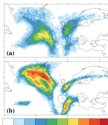
(a)
(b)
Figure 1. Total column probability of WCB occurrence (%), as
available during TNF. Probabilities are computed from ABL-started trajectories filtered for an ascent of 500 hPa in 48 h. Forecasts from
(a) 00:00 UTC, 15 October 2012 and from (b) 00:00 UTC, 17
Oc-tober 2012, both valid at 18:00 UTC, 19 OcOc-tober 2012. Compare to Fig. 3 in Schäfler et al. (2014).
lower probabilities close to the poles. Examples of the result-ing total columnp(WCB)field are shown in Fig. 1 and can also been found in Schäfler et al. (2014, their Fig. 3). Due to the described issues, the results should only be interpreted in a qualitative manner.
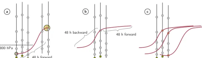
In 3-D, more complexity is added as the vertical extent of the grid cells also has to be taken into account. To elim-inate bias and sensitivity, one possibility is to assume an air parcel mass and geometry for the trajectory particles, as il-lustrated in Fig. 2a. In the example, the particle is associ-ated with a spherical air parcel. Given the required thermo-dynamic variables at the particle position at start timet0and gridding timet, the volume and thus radius of the parcel at
t can be computed and the overlapping grid points found. However, due to the large difference in vertical and horizon-tal scale of our grids (of the order of 100 km in the horizonhorizon-tal and 100 m in the vertical), the usage of spherical geometry re-quires the computation of a very large number of trajectories. Yet, geometry that reflects the different scales (for example ellipses, cylinders or simple rectangular boxes) is difficult to motivate physically. Also, usage of large air parcels neglects potential deformation of the parcels by the wind field.
An approach not requiring any such assumptions is to use domain-filling trajectories (in the following referred to as “DF-T method”). Here, we first specify the grid topology for
B. Next, as illustrated in Figs. 2b, c and 3, for every mem-ber and each grid point Bkj im , a trajectory starting on Bkj im
is computed. This way, we can be certain that each Bkj im is placed exactly on a trajectory and no assumptions about the
shape of the particle volume need to be made. After applying a WCB selection criterion to the trajectories, the bits of the grid points from which WCB trajectories were started are set. However, the approach requires increased computational re-sources. Seeding points are now required on all tropospheric layers and hence a larger number of trajectories is required. Also, trajectories additionally have to be computed backward in time to also capture those situations in which a WCB tra-jectory passes its seeding point in the ascent or outflow phase. Step (1) in the method description above is hence extended to also integrate the trajectories backward in time for1t hours from timet.
As an example, Fig. 3 shows results of selecting domain-filling trajectories that ascend more than 500 hPa in 48 h (Fig. 3a–c) and more than 600 hPa in 48 h (Fig. 3d–f). Note how the 30 % isosurface ofp(WCB)over the English Chan-nel almost vanishes with 600 hPa filtering (Fig. 3f).
In Sect. 3, we compare four DF-T and ABL-T set-ups with varying grid topology with respect to obtainedp(WCB)
and to computational demand. The comparison allows to find a set-up well-suited for usage in campaign forecasting. 2.3 Implementation
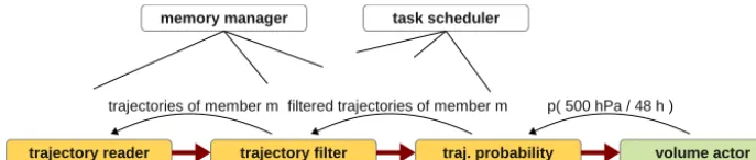
Trajectories computed with LAGRANTO are stored in NetCDF files. Trajectory selection and the computation of
p(WCB)take place in Met.3D and have been implemented in a number of modules in the Met.3D data processing pipeline described in Part 1, Sect. 4.2. Analogous to Fig. 10 in Part 1, Fig. 4 shows an example set-up. Separate pipeline modules are responsible for reading trajectory data from disk, filtering the data according to the selection criterion, gridding and probability computation. This architecture al-lows modules to be exchanged when, for example, data from a different trajectory model should be read or a different se-lection criterion should be applied.
Hardware permitting, parts of the pipeline (for example, trajectory selection) can be executed in parallel. Intermedi-ate results in the pipeline are cached by a memory manager. Both parallel execution and caching increase the interactivity of the system with respect to changing the selection param-eters1pand1t. For further details on the Met.3D pipeline architecture, we refer the reader to Part 1, Sect. 4.2.
Figure 2. Methods to computep(WCB). (a) ABL-T method using trajectories started in the atmospheric boundary layer and integrated 48 h forward in time. To get 3-D gridded information on WCB location, an air parcel volume needs to be assumed for each particle so that grid points overlapping with the volume can be determined. (b) DF-T method using domain-filling trajectories started from every grid point of thep(WCB)grid and integrated both 48 h forward and backward in time. No volume has to be assumed as selected WCB trajectories are located exactly on grid points (c).
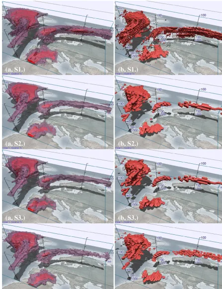
Figure 3. Derivation ofp(WCB)with DF-T set-up (S3). (a, d) Trajectories started at 18:00 UTC, 19 October 2012, computed with wind fields from the ensemble control forecast from 00:00 UTC, 17 October 2012, integrated forward and backward in time for 48 h each. Trajectories are selected according to an ascent of (a–c) 500 and (d–f) 600 hPa in 48 h. Colour encodes altitude (hPa). (b, e) Volume rendering of the binary gridB, representing the start positions of the selected trajectories. (c, f) Probability of WCB occurrence derived from all 51 members of the ensemble. The red opaque isosurface shows 30 % probability, the purple transparent isosurface 10 % probability. Vertical axes are labelled with pressure altitude (hPa).
fulfils the selection criterion. The data volume that needs to be loaded can be largely reduced by pre-computing the max-imum pressure change1pfor a range of time intervals1t. Now, for a given1t, only the maximum1pfor each trajec-tory (i.e. grid point) needs to be read. The selection process is reduced to comparing each trajectory’s 1p to the given threshold value. This way, we are able to provide an interac-tively adjustable selection criterion to the user.
3 Choice ofp(WCB)method and grid spacing for forecasting
To use ap(WCB)method for forecasting during a campaign, a number of criteria need to be fulfilled:
Figure 4. Sample Met.3D data processing pipeline to visualizep(WCB), depicted analogous to Fig. 10 in Part 1. Different pipeline modules (yellow) are responsible for reading and selecting trajectories, and for computing thep(WCB)field. In the example, a volume actor (green; for details see Part 1, Sect. 3) visualizes the resultingp(WCB)data. A request for the probability of occurrence of trajectories, emitted by the volume actor, triggers further requests up the pipeline. Intermediate results are cached by the memory manger, connected to each pipeline module (indicated by the black lines). Pipeline execution can be parallel and is controlled by a task scheduler, also connected to all pipeline modules (for details see Part 1, Sect. 4.2).
b. the amount of trajectory data needs to be small enough to be handled interactively in Met.3D;
c. the grid spacing needs to be fine enough to capture the important features that are present in a “best-possible” forecast.
3.1 Evaluated set-ups
We evaluate four different set-ups with respect to the given criteria:
S1. As the “best-possible”p(WCB)forecast, we use a DF-T set-up with trajectories computed on the ECMWF ENS wind fields at the highest available grid spacing (T639L62 spectral resolution, horizontally interpolated by MARS to a regular grid of 0.25◦×0.25◦ in lati-tude and longilati-tude, with 62 hybrid sigma-pressure lev-els in the vertical). Care must be taken with respect to the choice of the Bm andp(WCB)grids. A straight-forward choice is to use the ECMWF grid on which the wind fields are available. However, the vertical po-sition of the grid points on all but the uppermost hy-brid sigma-pressure levels depends on the surface pres-sure field (Untch and Hortal, 2004, also cf. Part 1, Sect. 4.1), which varies between ensemble members and time steps. Hence, if for a given time step the individual members’ wind grids are used for theBm, the problem described in Part 1, Sect. 5, arises: the grid points are lo-cated at different vertical positions across the ensemble, and hence an error is introduced when computing the probability. To avoid this problem while staying as close as possible to the ECMWF grid, we use the grid defined by the time step’s ensemble minimum surface pressure for theBmof all members. The minimum surface pres-sure is chosen to enpres-sure that all grid points are located above the surface (if the mean surface pressure is used, grid points in the lowest levels can be located below the surface in some members). We focus on a vertical region of interest of up to approximately 100 hPa and for the
Bmandp(WCB)grids discard the model levels above this elevation (retaining the lower 52 levels).
S2. The same set-up as (S1), but with horizontal wind field,
B, and p(WCB)grid spacing reduced to 1◦×1◦. As in (S1), the lower 52 vertical levels are used forB and
p(WCB).
S3. The same set-up as (S2), but withBandp(WCB)grids defined by a constant surface pressure of 1000 hPa, not by the ensemble minimum surface pressure. The wind forecast data remain as in (S2). The advantage of this set-up is that thep(WCB)grid can be interpreted as a structured pressure level grid and thus be visualized much more efficiently (Part 1, Sect. 4.3). This way, the interactivity in Met.3D can be improved. The drawback, however, is that some of the lower-level grid points are now located below the surface and become invalid. This reduces the vertical grid spacing in the lower tropo-sphere above mountainous terrain.
S4. An ABL-T set-up using a gridB that is regular in the horizontal with a grid spacing of 1◦×1◦as in (S2) and (S3). In the vertical, the grid is regular in pressure with a grid spacing of 10 hPa. This spacing is of the order of the average spacing of the model level grids used in (S2) and (S3), and results in a comparable number of vertical levels in the region of interest (90 levels between 1000 and 100 hPa). Usage of a regular pres-sure level grid can be motivated physically; from hydro-static balance (e.g. Wallace and Hobbs, 2006, Sect. 3.2), we know that for a column of air with constant mass
mthe difference in pressureδp between top and bot-tom boundary of the column stays constant with height:
when rising at constant latitude. The artefact of decreas-ing grid cell areaAtowards the poles remains, though. For trajectory integration, the same forecast data as in (S2) and (S3) are used.
For all trajectory computations, LAGRANTO is driven with ECMWF ENS forecast data at 6 h time steps. The model internally uses a 30 min time step for the integration, trajec-tory positions are output at 6 h intervals.
3.2 Set-up comparison
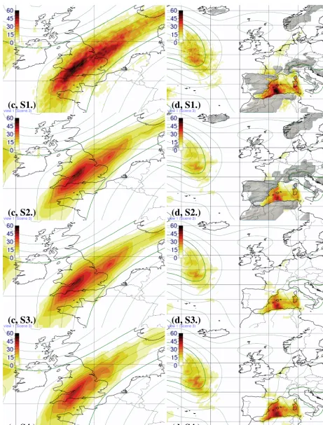
In terms of computational resources, set-up (S1) is the most demanding configuration. On our test system (six-core Intel Xeon running at 2.67 GHz; 24 GB RAM; 512 GB solid state drive), the computation of the trajectories of a single time step takes about 50 CPU minutes per member. The data out-put for a time step of all members, stored in binary NetCDF format, amounts to approximately 38 GB. While such simu-lations are feasible for research settings, they are not suited for forecasting. For set-ups (S2) and (S3), the number of tra-jectories decrease by a factor of 16. The time required to compute the trajectories reduces to about 3 CPU minutes per time step and member, about 2.4 GB of trajectory data are produced per time step for the entire ensemble. With the current ENS size of 51 members, this setting is feasible for forecasting if a small compute cluster is available. For set-up (S4), the time further reduces to about 1 CPU minute and data volume reduces to approximately one GB.
In Figs. 5 and 6, the four set-ups are compared by means of four typical visualizations of the Met.3D workflow: (a) the volume rendering of p(WCB) isosurfaces already used in Fig. 3c, (b) a volume rendering of WCB features in forecast member 12 (as captured by the binary gridB12), (c) a hori-zontal section at 410 hPa through the ascent region associated with precipitation and (d) a horizontal section through the inflow region at 950 hPa. The TNF forecast case of 19 Oc-tober 2012 that already served for the examples in Part 1 is used. The main features (cf. Fig. 1 in Part 1: inflow over the Mediterranean Sea, ascent over the English Channel and southern England, outflow over Scandinavia and Russia, as well as a strong ascent associated with former Hurricane Rafael over the North Atlantic) are well represented by all set-ups. However, in the regions of maximump(WCB), set-ups (S2) and (S3) predict probabilities that are decreased by about 10 % compared to the “reference” set-up (S1). This is visible in the smaller extent of the 30 % isosurface in Fig. 5a as well as in the horizontal sections (Fig. 6c, d). Also, single member WCB structures are more solid in set-up (S1), as illustrated in the 3-D view of the binary volume of member 12 (Fig. 5b). The decrease is caused by the lower horizontal grid spacing of the driving wind fields, in which fewer trajec-tories experience strong ascent – potentially due to smoothed vertical velocities. Nevertheless, set-ups (S2) and (S3)
cap-ture the shape and location of thep(WCB)features equally well as (S1).
The differences between set-ups (S2) and (S3) are negli-gible. While virtually no differences can be found in the vi-sualizations of the WCB ascent at 410 hPa (Fig. 6c), the dif-ferences become more pronounced in the lower atmospheric layers (Fig. 6d). This can be explained with the grid topol-ogy: at higher altitudes, the elevation of the model levels be-comes increasingly independent of surface pressure (cf. Part 1, Sect. 4.1) and hence the difference in thep(WCB)grids vanishes. However, even at low altitudes the observed differ-ences inp(WCB)remain within a few percent.
The bottom rows of Figs. 5 and 6 show the results for the ABL-T set-up (S4). Despite the crude assumption with re-spect to air parcel geometry, the majorp(WCB)features are captured well. However, this set-up tends to predict slightly higher probabilities compared to (S2) and (S3) in the atmo-spheric boundary layer, and slightly lower probabilities at higher altitudes.
Results for other time steps are similar (not shown). We conclude that from the presented candidates, set-ups (S3) and (S4) are best suited to be used in a forecast setting. While showing small differences with respect to the absolute pdicted values, both capture the shape and locations of re-gions of elevatedp(WCB). Also, both are feasible to com-pute in less than an hour and the results can, due to the struc-tured vertical grid layout, be visualized more efficiently than the results computed by the set-ups based on hybrid sigma-pressure vertical coordinates (cf. Part 1, Table 2)1.
4 Probability region contribution
The methods introduced so far allow one to visualize the computedp(WCB)fields and to find regions in which the occurrence of a WCB is most likely. However, it remains an open question how the magnitudes of the displayed proba-bilities should be interpreted. A distinct property of the ex-amples presented in Sect. 3 are relatively low probabilities. For instance, in Fig. 3c maximum values only reach about 30 %. As mentioned in the introduction, such low magnitudes can have two causes: either indeed only 30 % of all ensem-ble members predict the WCB event, or large spatial varia-tion of the features in the individual members causes only marginal overlap and thus low probabilities. Also, noise in the individual binary volumes can cause empty grid cells in the features and decrease probability values. Interpreting the data correctly and being able to distinguish between these 1To provide an order of magnitude of the rendering times, using
(c, S1.)
(d, S1.)
(c, S2.)
(d, S2.)
(c, S3.)
(d, S3.)
(c, S4.)
(d, S4.)
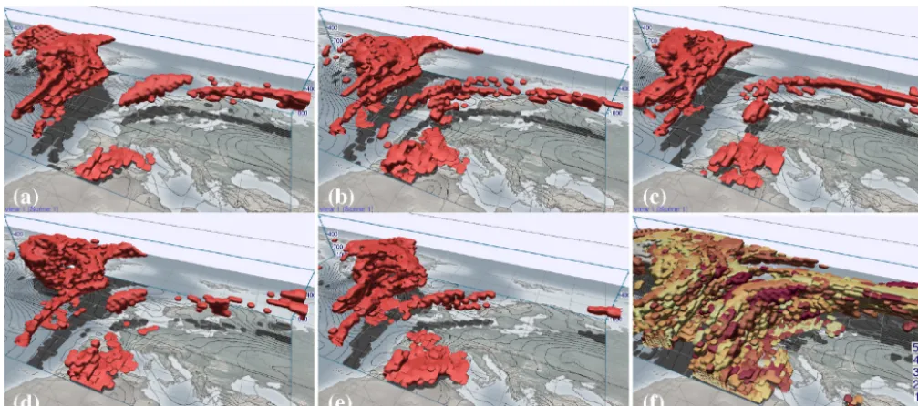
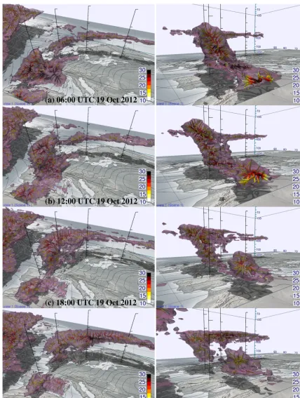
Figure 7. WCB features (binary gridsBm) of further membersmof the forecast shown in Fig. 3b. Members (a) 2, (b) 4, (c) 34, (d) 36 and
(e) 42. Note that location and shape of the WCB features vary strongly. (f) WCB features of all 51 members of the ensemble, visualized
in a single image and distinguished by colour (colour coding denotes member number). Black contour lines in all images show sea level pressure of the corresponding member (of the ensemble mean in f).
causes is very important for making decisions on potential flight routes.
The issue can be approached by looking at the individ-ual ensemble members, as illustrated in Fig. 7. While due to limited print space, Fig. 7 only shows a small selection of members, we indeed find that much more than 30 % of the members predict a WCB feature. However, it is difficult for a human user to remember how many of the 51 members showed a WCB feature. Visualizing the WCB features of all members in a single view (Fig. 7f) results in massive clutter and, thus, does not reveal insight.
We are interested in the following information: given a re-gion bounded by a probability isosurface, how many individ-ual ensemble members predict a WCB feature that overlaps with this region and that, thus, contributes to the probability value at any of the grid points inside the isosurface? To de-termine this number of members, we propose a method that applies region growing to identify the grid points inside the isosurface, then uses the members’ binary gridsBmto deter-mine which members have contributed. To efficiently make use of theBm, we condense the binary grids into bitfields that are stored together with the probability volume. For the cur-rent example and for the 51 members of the ECMWF ensem-ble, each grid point p(WCB)kj i is augmented by a bitfield stored in a 64 bit integer variable (1 bit for each member). The bitfields are generated during evaluation of the probabil-ity criterion (in this case, step (3) in Sect. 2).
Figure 8 illustrates the approach. In a hypothetical ensem-ble of ten members, nine members predict a WCB feature
Figure 8. Schematic 2-D example of a case in which many
ensem-ble members predict a WCB feature but spatial variation causes low probability values. Consider an ensemble of ten members, of which nine members predict a WCB feature (depicted by the differ-ent coloured and numbered lines). In the example, only a maximum of three features overlap in any grid cell (resulting in a maximum probability of 30 %; red grid cells). By storing the indices of all members that contribute to a given grid cell, our method is able to determine the members that contribute to a probability region. In the example, eight members (that is, 80 %) contribute to the red region. The grey grid cells illustrate the 10 % region.
of the identified points with a bitwise ”or”-operation reveals that in total, members 1, 2, 3, 4, 5, 6, 8 and 9, thus 80 % of the ensemble, contribute to the region. We hence know that much more than 30 % of all members predict a WCB. The information is stored for each of the identified grid points in a separate data field, the “contribution volume”. It needs to be recomputed every time the probability isovalue changes. For example, applying the algorithm to the white 10 % region in Fig. 8 yields a contribution of 90 %.
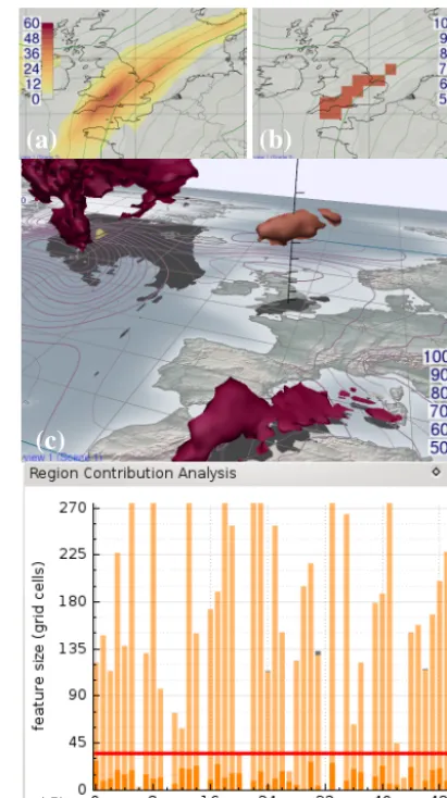
The contribution volume can be used in visualizations of
p(WCB)to colour a probability isosurface according to the number of members that contribute. Figure 9 shows the ap-plication of the method to the WCB forecast from Fig. 3c, set-up (S3). Whenever an isosurface point is identified and visualized (cf. Part 1, Sect. 4.3, for the employed raycast-ing algorithm), the eight data points that enclose the isosur-face position are sampled. Since the isosurisosur-face value is in-terpolated from these eight points, at least the point with the maximum probability value is located inside the isosurface, and the point with the lowest value is located outside the iso-surface (otherwise no crossing could be found between the points). Thus, by sampling the contribution volume at the grid point with the maximum value (and exploiting the fact that all grid points of a contiguous structure in the contribu-tion volume carry the same value) the number (or percentage) of contributing members can be obtained. Indeed, Fig. 9c shows that about 85 % of the example’s ensemble members contributed to the 30 % isosurface – an immediate hint to the forecaster to have a closer look at the predicted structure.
In addition, region growing can be applied to yield infor-mation on how many disjoint WCB features contribute from a particular member, and how the sizes of these features com-pare to the size of the region bound by the probability isosur-face. The diagram in Fig. 9d is displayed by Met.3D when the user selects an isosurface with the mouse pointer. It shows the sizes of the WCB features in the individual members in a stacked box plot. The size of the probability isosurface is displayed by the red line. Single features are divided into solid bars, depicting the fraction of the feature that overlaps with the probability isosurface, and a transparent bar, depict-ing the full size of the feature. If more than one feature con-tributes from a given member, each disjoint feature is shown in a different colour. For the example in Fig. 9, this informa-tion reveals further insight: first, most members contribute exactly one contiguous feature; second, these features are for the most part substantially larger than the isosurface region (also compare the size of the probability isosurface to the WCB features in Fig. 7). We infer that most members’ fea-tures indeed represent WCB events. A WCB is hence very likely to occur.
Of course, the method can also be applied to probabil-ity fields other thatp(WCB); similarly low probabilities can also occur for features derived from other NWP fields.
(a)
(b)
(c)
(d)
Figure 9. Application of the region contribution algorithm to the
WCB forecast from Fig. 3c. (a) Horizontal section ofp(WCB)at 415 hPa over southern England (colour coding in %). (b) Grid boxes that intersect with the 415 hPa surface and that exceed the isosur-face threshold of 30 % (the red isosurisosur-faces in Fig. 3c), coloured by the percentage of contributing members as identified by the region growing algorithm (colour coding in %). Green contour lines in (a) and (b) show ensemble mean geopotential height. (c) The 30 % iso-surfaces of Fig. 3c coloured by the percentage of contributing mem-bers. Purple contour lines show ensemble mean sea level pressure.
(d) Size (in grid cells) of WCB features in the members contributing
to the 30 % isosurface above southern England. If multiple features contribute from a given member, they are stacked using different colours (in the example, small secondary features exist in members 24, 31 and 46). The bar of each feature is divided into total feature size (light colour) and the fraction of the feature that overlaps with the 30 % isosurface (solid colour). The red horizontal line marks the size of the 30 % isosurface.
5 Case study
Figure 10. Time sequence of (left) horizontal section with contour lines of geopotential height and filled contours of wind speed (ms−1) at 250 hPa, (middle) jet stream (opaque isosurface 50 ms−1, transparent isosurface 30 ms−1, and black contour lines of sea level pressure) and (right) clouds (opaque isosurface cloud cover fraction of 0.7, transparent isosurface cloud cover fraction of 0.2, and black contour lines of sea level pressure). Colour coding in the right panel denotes cloud elevation in hPa. Deterministic forecast from 00:00 UTC, 15 October 2012, valid at (a) 18:00 UTC, 18 October 2012, (b) 18:00 UTC, 19 October 2012 and (c) 00:00 UTC, 21 October 2012.
demonstrates how Met.3D can be used in practice. The pre-sented case study revisits the TNF forecast case for 19 Oc-tober 2012, a case that has already been used in the previous sections and in Part 1 and that is also discussed in Schäfler et al. (2014). We supplement the case study with a video ac-companying this paper, as it helps convey the full value of Met.3D’s interactive 3-D visualizations. The video contains this section’s static figures, as well as additional content, in animated form. It is intended to be used side-by-side with the paper. Start times for the video are provided throughout the following text. To compute p(WCB), set-up (S3) from Sect. 3 is used.
Assume the forecast activities to take place on Monday, 15 October 2012. The ensemble and deterministic predic-tions initialized at 00:00 UTC on that day, as well as the pre-ceding model runs, are available to the forecaster (in the fol-lowing, we abbreviate forecast valid times as “12Z/19” for 12:00 UTC, 19 October 2012, and forecast initialization (or base or run) times as “IT00Z/15” for 00:00 UTC, 15 October
2012). We are interested in areas that favour WCB develop-ment in central Europe, being reachable with the Deutsches Zentrum für Luft- und Raumfahrt (DLR) Falcon aircraft from the campaign base in Oberpfaffenhofen, southern Germany. Due to requirements from air traffic authorities, potential flight routes need to be announced at least three days in ad-vance of a flight. Hence, our aim is to explore the atmo-spheric situation in order to evaluate suitable flight condi-tions towards the end of the week.
5.1 Weather situation
horizon-tal section of wind speed and geopotential height (initially placed at jet stream level at 250 hPa), 3-D isosurfaces of wind speed and 3-D isosurfaces of cloud cover. We explore the time period from Wednesday, 17 October, to Sunday, 21 Oc-tober. Figure 10 shows screenshots of the individual views at three selected time steps. To capture the 3-D spatial struc-ture of the jet, the isosurfaces of wind speed are visualized at 30 and 50 ms−1. Cloud cover is visualized by isosurfaces at 0.2 and 0.7, the latter coloured by elevation. Both 3-D views contain contour lines at surface level showing the mean sea level pressure. The video shows the Met.3D window with the full time animation.
A number of events of interest to our objectives can be observed: a distinct trough over the Atlantic moves eastward and narrows over time. At the same time, high pressure over central and eastern Europe intensifies. At upper levels, a pro-nounced jet stream extends from Spain over southern Eng-land to Scandinavia, causing strong winds over western Eu-rope blowing from a southerly direction. On the leading edge of the trough, upper level cirrus clouds are embedded in the jet, whereas upstream, i.e. on the rear side of the trough, only scattered low-level clouds are present. Further upstream (south of Greenland in Fig. 10), the large-scale flow and cloud field are perturbed by the extratropical transition of for-mer Hurricane Rafael (cf. Fig. 1 in Part 1; cloud field visible in the video). It approaches from the south and transforms into an extratropical cyclone. The leading edge of the trough, covering France and southern England, would be well reach-able with the Falcon.
Before we explore further forecast data, we obtain infor-mation about the uncertainty of the forecast (forecast ques-tion B). First, we check the consistency of the deterministic forecast by comparing the currently used forecast (IT00Z/15) to the two previous runs from IT12Z/14 and IT00Z/14. The video (at 00:36 min) shows how the forecast runs are tog-gled for the forecast valid at 18Z/19. While the IT00Z/15 and IT12Z/14 runs show a fairly consistent situation, the trough is much broader in the IT00Z/14 forecast. Also, the strong jet on its leading edge has a different shape and is located fur-ther east and furfur-ther north. For specifying a flight route, this spatial uncertainty is an important factor.
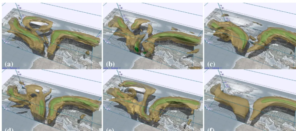
To get a more comprehensive picture, we explore the en-semble forecast of IT00Z/15 for occurrence, location and in-tensity of trough and jet in the individual members. Figure 11 shows selected ensemble members and the ensemble mean of the jet stream visualization for the forecast valid at 18Z/19 (the animation over the members is contained in the video at 01:14 min). The jet over Europe is present in all mem-bers with similar intensity. However, we observe variation in shape and location that is in part stronger than the difference between the IT00Z/14 and IT00Z/15 deterministic forecasts. Nevertheless, the majority of the members predict a compa-rable jet structure over Europe. This also becomes apparent in the ensemble mean, which despite averaging features a jet core of over 50 ms−1. In contrast, the variation observed in
the jet structure further upstream over the central North At-lantic is larger, indicating that the predicted evolution of the extratropical transition of Hurricane Rafael is very uncertain. Here the 50 ms−1signal is smoothed out in the mean.
In summary, we conclude that at least parts of the re-gion approximately covering France, southern England and Benelux will be located on the downstream side of the trough.
5.2 Warm conveyor belt occurrence
Next, we examine thep(WCB)data to determine whether a suitable WCB event is likely to occur in our region of inter-est (forecast quinter-estion C). Figure 12 shows selected time steps from the IT00Z/15 forecast; the corresponding animation is shown in the video at 01:55 min. We choose an initial se-lection criterion of1p=500 hPa in1t=48 h and visualize the predicted fields with a 3-D isosurface of a low probability (10 %). To track the temporal evolution of thep(WCB)field inside the isosurface (in particular the evolution of the max-ima), the 3-D normal curves proposed in Part 1, Sect. 3.4, are used2.
Indeed, we find that on both 18 and 19 October, WCB air masses are likely to ascend on the leading edge of the trough over France and southern England. These air masses are po-tentially of interest to a research flight. Since the normal curves reveal larger probabilities on 19 October, we focus on this day. At 12Z/19 (Fig. 12b) and 18Z/19 (Fig. 12c), the ascent signal is most apparent in the prediction. At 00Z/19 and 06Z/19 (Fig. 12a), the air mass is still close to the sur-face and too far south to be reached by a single Falcon flight. At 00Z/20 (Fig. 12d) and 06Z/20, the air mass has reached upper levels and WCB activity is dominated by outflow. For the campaign objectives, the time around 12Z/19 and 18Z/19 is most interesting to us: the air is ascending and hence me-teorologically active (precipitation is associated with the as-cending phase of a WCB), and it is located in an area that can be well reached by the Falcon. The 3-D visualization al-lows one to judge the vertical extent, shape and elevation of the region of high probability. The normal curves, coloured by probability, reveal that the maximum values ofp(WCB)
on 19 October are of the order of 20 to 30 %. By moving the camera and using vertical poles, we see that the region en-closed by the 10 % isosurface is tilted westwards (left column of Fig. 12; video at 02:29 min). At 18Z/19, the maximum is located at around 400 hPa.
Due to the low magnitudes ofp(WCB), we next intend to clarify (a) whether indeed only a few ensemble mem-2Normal curves are well-suited in this case to obtain an overview
Figure 11. Navigation through the ensemble. Members (a) 27, (b) 33, (c) 37, (d) 43, (e) 45 and (f) the ensemble mean of horizontal wind
speed (forecast from 00:00 UTC, 15 October valid at 18:00 UTC, 19 October 2012). Shown are the 50 ms−1(green opaque) and 30 ms−1 (yellow transparent) isosurfaces. Black contour lines show sea level pressure.
bers predict the WCB, and (b) how the predicted probability changes with a changing selection criterion (forecast ques-tion D). Figure 13a shows a screenshot of Met.3D with the region contribution analysis (Sect. 4) applied to the forecast valid at 18Z/19 (video at 02:42 min). A 20 % isosurface is used to capture the regions of maximum predictedp(WCB). Indeed, for both 12Z/19 (not shown) and 18Z/19 the analy-sis confirms that over 85 % of the ensemble members have contributed to the 20 % probability region over the English Channel. The difference between 20 and 85 % indicates large spatial variation in the ensemble. Also, the histogram (on the right side of Fig. 13a) shows that the majority of individual WCB features that overlap with the 20 % isosurface cover a larger volume than the resulting probability region itself. This implies that the regions that experience ascent in the in-dividual members are larger than the region enclosed by the isosurface. To validate these findings, we animate over the individual members (Fig. 13b, c, and d; video at 03:16 min). Indeed, almost all members predict a WCB feature on the leading edge of the trough. However, as expected, the vari-ability in shape and location of the predicted features is very large. In addition to members in which the WCB air ascends at 18Z/19, members in which the air is already in the outflow stage (elongated features at jet stream level) or still in the inflow stage (close to the surface) are equally present. This indicates additional temporal uncertainty. Hence, while there seems to be a good chance to sample WCB air on 19 October in the region covering western France to southern England, the location in space and time of the WCB ascent is still un-certain in the IT00Z/15 forecast.
To judge the strength of the predicted ascent, we mod-ify the trajectory selection criterion. Figure 14 (video at 03:38 min) shows how the predictedp(WCB)changes with
1p. By decreasing 1p (Fig. 14a), we can confirm a high likelihood of ascending air masses in the region of interest3; the probability increases with decreasing1p. Increasing1p
(Fig. 14b) reduces the predicted probabilities. However, the location of the maximum remains at the same position. The region in which high probabilities for ascending air masses are forecast is hence also the region in which the strongest updrafts occur.
5.3 WCB characteristics
The next goal is to characterize the predicted ascent with re-spect to related atmospheric processes (forecast question E). We take a closer look at the WCB trajectories of the ensem-ble control run and visualize the trajectory particle positions at single time steps. Animation over the time steps of the tra-jectories computed forward and backward from 18Z/19 re-veals that the air that at 18Z/19 has ascended to the region over the Channel originates from the ABL over the western Mediterranean Sea and northwestern Africa around 18Z/18 (Fig. 15a, video at 04:10 min). It is lifted over Spain in the early hours of 19 October and over the course of the day continues its ascent over western France, the Channel and southern England (Fig. 15b, c). By vertically shifting a hori-3Note that the normal curves are again advantageous for this
Figure 13. Region contribution analysis applied to the ensemble forecast from 00:00 UTC, 15 October 2012, valid at 18:00 UTC, 19
Octo-ber 2012. (a) Screenshot of the Met.3D configuration; 20 % isosurfaces ofp(WCB)are coloured by the percentage of contributing members. The contribution distribution of the feature over southern England is shown in the histograms on the right side of the window (feature size in (top) grid cells and (bottom) 103km3; see Fig. 9 for details on the diagram). (b–d) WCB features (binary gridsB) as predicted by the individual ensemble members (b) 2, (c) 9 and (d) 19. Purple surface contours in (a) and black surface contours in (b–d) show sea level pressure.
zontal section of geopotential height and equivalent potential temperature of the deterministic forecast at 18Z/18 (similar to the ensemble control but chosen here for its added detail), we discover a cyclone over the northern British Isles, and a weaker surface low located on the west coast of France (Fig. 15d; video at 04:28 min). South of Spain, warm and moist air (high equivalent potential temperature) is advected northward. This air mass represents the WCB inflow region; it is subsequently lifted by the WCB. In contrast, on the rear side of the trough, colder and drier air masses over the eastern Atlantic are transported southward to Spain. Over the follow-ing 24 h, the cyclone over the British Isles remains stationary, the weaker surface low moves towards Norway (Fig. 15e, f; video at 04:52 min). Animation over the ensemble members reveals that most other members predict similar ascents orig-inating from the western Mediterranean Sea and northwest-ern Africa. Figure 16 reproduces the visualization of Fig. 15c for the members shown in Fig. 13b, c, and d. The trajectory particles that represent the WCB air masses are lifted along similar paths. However, the temporal evolution of the WCBs differs in the members. At 18Z/19, the air masses are at dif-ferent stages of their ascent.
Figure 14. Adjusting the filter criterion for thep(WCB)forecast shown in Fig. 12c (forecast from 00:00 UTC, 15 October 2012, valid at 18:00 UTC, 19 October 2012). Filter criterion of (a) 400 hPa and (b) 550 hPa in 48 h (in Fig. 12c a criterion of 500 hPa in 48 h is used). The purple transparent isosurfaces show a probability of 10 %. Normal curves inside the isosurfaces are coloured by proba-bility (%). Black contour lines show ensemble mean sea level pres-sure.
5.4 Potential flight segments
Given the findings from the previous subsections, we inter-pret thep(WCB)maximum as the most likely location for the predicted WCB event and draft potential flight segments. Figure 18 shows the corresponding Met.3D configuration. For 12Z/19 and 18Z/19, we slide a horizontal section trough the p(WCB)volume to determine precise locations of the maxima (video at 05:42 min). At 12Z/19, maximum proba-bilities are located above the Pyrenees at low levels, in the Bordeaux area between 700 and 600 hPa, and south of Brit-tany around 400 hPa; 6 h later, the maximum is most promi-nent above southern England at altitudes around 400 hPa. A vertical section is used to explore potential flight segments. It allows one to estimate at which elevation a flight should take place, and, by moving the section, to quickly assess how spatially relocating the leg will impact the expected measure-ments. In the given case, the 2-D sections suggest flight legs at 12Z/19 over France at elevations between 800 and 600 hPa
(WCB ascent) and at 18Z/19 over southern England at eleva-tions around 400 hPa (WCB outflow)4.
However, given the uncertainty in the temporal evolution of the WCB (previous section), we need to carefully monitor developments in subsequent forecast runs. Figure 19 (video at 07:38 min) shows the predictions for 18Z/19 for forecast runs subsequent to the IT00Z/15 run. Over the next 2 days, the ensemble predictions converge toward higherp(WCB)
over the English Channel and southern England. The eleva-tion of the predicted maximum inp(WCB)remains approx-imately constant. Indeed, the research flights conducted dur-ing TNF showed that the targeted WCB occurred as predicted (Schäfler et al., 2014).
6 Conclusions
Motivated by the forecast requirements of the T-NAWDEX-Falcon 2012 campaign, we have demonstrated the feasibility of applying interactive 3-D ensemble visualization to fore-casting warm conveyor belt situations during aircraft-based field campaigns. The article extends our work presented in Part 1, in which we have introduced the new open-source 3-D ensemble visualization tool Met.3D. In the present paper, we have proposed methods to compute and to visually analyse 3-D probabilities of WCB occurrence. The techniques have been integrated into Met.3D and are part of the released ver-sion 1.0 (see Part 1, Sect. 6, for information on code avail-ability). A case study, revisiting a forecast case that occurred during T-NAWDEX-Falcon, has demonstrated how the meth-ods introduced in the two papers can be used for practical forecasting.
Following the literature, our methods detect WCBs by means of Lagrangian particle trajectories. By computing tra-jectories for each member of the ECMWF ensemble forecast, a distribution of WCB features is obtained from which prob-abilities of occurrence can be derived. We have discussed different approaches to trajectory seeding and gridding, and have shown that probabilities derived from trajectories com-puted at a horizontal grid spacing of 1◦in latitude and lon-gitude capture the same WCB structures as trajectories com-puted at a higher grid spacing of 0.25◦. A proposed visual analysis method supports the interpretation of the probabil-ity fields. The method facilitates fast visual estimation of the number of ensemble members that forecast a WCB feature in a region of interest bounded by a probability isosurface. In particular for situations in which the magnitude of observed probabilities is low, the method helps to distinguish the case 4During TNF, we did not have the verticalp(WCB) informa-tion available. We placed the flight along a horizontally pre-defined flight leg over France which appeared to fit well with the 2-D
Figure 15. (a–c) Particle positions of the (backward) WCB trajectories of the ensemble control forecast, started at 18:00 UTC, 19
Octo-ber 2012 and computed on the forecast initialized at 00:00 UTC, 15 OctoOcto-ber 2012. Colour codes pressure elevation in hPa. (d–f) Horizontal sections of geopotential height (contour lines), wind barbs and equivalent potential temperature (colour coded in K) of the deterministic forecast from 00:00 UTC, 15 October 2012 at 950 hPa. Forecasts are valid at (a, d) 18:00 UTC 18 October 2012, (b, e) 06:00 UTC, 19 October 2012 and (c, f) 18:00 UTC, 19 October 2012.
Figure 16. The same as Fig. 15c, but for the ensemble members (a) 2, (b) 9 and (c) 19. Also compare to the visualizations of the corresponding
binary gridsBshown in Fig. 13b–d.
in which only few members predict a WCB but at approxi-mately the same location, from the case in which many mem-bers predict a WCB but the spatial variation is high. The method can be applied to probabilities of other features as well.
With Met.3D and the proposed WCB methods, we are now able to analyse ensemble prediction data in a way previ-ously impossible. Three of us (M. Rautenhaus, C. M. Grams, A. Schäfler) have been actively involved in forecasting dur-ing aircraft-based field campaigns. With respect to the case study and our experience in research flight planning, we note a few conclusions from our work, reflecting the authors’ opinions.
1. Combination of 2-D and 3-D visualization methods gives a more complete picture of the forecast
atmo-sphere; 3-D elements can depict different aspects of the data than horizontal and vertical 2-D sections alone. For example, usage of isosurfaces and normal curves allows for very fast initial judgement of the predicted WCB sit-uation. However, we would not want to abandon the fa-miliar 2-D sections; for many tasks (obtaining quantita-tive information, visualizing multiple forecast parame-ters in the same plot, analysing the vertical structure of the atmosphere along a flight segment) they are superior to 3-D methods. If 3-D visualization is used, achieving good spatial perception is important, as we have dis-cussed in Part 1.
vari-(a)
(b)
Figure 17. (a) Vertical section of potential vorticity (colour coding in PVU; red colours in the left plot mark the 2 PVU surface and thus
the dynamic tropopause), potential temperature (grey contour lines), liquid and ice water content (blue and green contour lines). (b) Vertical section of cloud cover fraction (colour coding) and equivalent potential temperature (red contour lines). Black surface contour lines in both
(a) and (b) show sea level pressure. Deterministic forecast from 00:00 UTC, 15 October 2012, valid at 18:00 UTC, 19 October 2012.
Figure 18. Planning potential flight legs with Met.3D (ensemble forecast from 00:00 UTC, 15 October 2012, valid at 18:00 UTC, 19
Oc-tober 2012). The large view in the middle shows a vertical section ofp(WCB)(colour scale in %), potential temperature (black contour lines), liquid and ice water content (blue and white contour lines). Purple surface contours show ensemble mean sea level pressure. The small view on the upper right shows a vertical section of potential vorticity (same colour coding and contour lines as in Fig. 17a). The small view on the lower right shows a horizontal section at 390 hPa, showingp(WCB)(same colour scale as in the large view) and contour lines of ensemble mean geopotential height. The maximump(WCB)along the proposed leg can be found over southern England at around 400 hPa. The vertical section of PV shows how a flight at that altitude, going westward, would penetrate the tropopause shortly after sampling the WCB.
ables. For the isosurfaces of wind speed and WCB prob-ability used in the case study, 3-D visualization is well-suited. For variables that highly fluctuate in space (as is often the case for variables depending on moisture, such as relative humidity), isosurfaces are problematic. For these cases, additional methods that help the user focus on the regions and features of interest will need to be developed.
(a)
(b)
Figure 19. Convergence ofp(WCB)with decreasing forecast lead time. Forecasts from (a) 12:00 UTC, 15 October 2012 and (b) 12:00 UTC, 16 October 2012, valid at 18:00 UTC, 19 October 2012. Filter criterion is 500 hPa in 48 h. Isosurfaces show 30 % (red opaque isosurface) and 10 % (purple transparent isosurface). Black surface contours show ensemble mean sea level pressure. The fore-cast from 00:00 UTC, 17 October 2012 is shown in Fig. 3c.
of uncertainty (animation over the ensemble, compari-son of different forecast base times) and of sensitivity (changing a parameter that affects a displayed statistical quantity).
However, we find that while interactivity enables the user to quickly visualize a large amount of data, the user is also confronted with many more images than they would be if they were restricted to, for example, a lim-ited number of horizontal sections. Here, as Trafton and Hoffman (2007) suggest, a virtual “sketchpad” that cap-tures elements discovered by the forecaster and that al-lows him/her to represent his/her “mental model” of the atmosphere would be useful. The sketchpad could also be used to communicate the findings to colleagues, a common challenge during campaigns.
3. Our methodology to predict probabilities of WCB occurrence illustrates challenges of feature-based ap-proaches to analyse ensemble data. Our region contri-bution approach helps to interpret the derived probabil-ities; however, further work will be useful. For exam-ple, we would like to automatically obtain information
about how features in different members correspond to each other: do other members predict the same situation but shifted in space or in time? Such information would allow one to identify different scenarios forecast by the ensemble, and uncertainty could be differentiated with respect to space and time. Detection and visualization of further 3-D cyclonic features would also be very use-ful. For a single member we could see at a glance, for example, which WCB transports which air mass along which route, driven by which cyclone and in relation to which front and jet stream. How to meaningfully visu-alize such features for an entire ensemble to depict their uncertainty is an open research question.
4. A drawback of the Met.3D visualization approach is that since it uses the complete ensemble data set, in-teractive usage requires the forecast data to be avail-able on the local hard drive. For field campaigns based at remote locations, this is not feasible. In these cases, web based approaches such as DLR’s Mission Support System (Rautenhaus et al., 2012) might be the better choice. Alternatively, dedicated ensemble compression schemes might enable more efficient remote handling, or remote visualization solutions such as VirtualGL5 could be used to locate data and visualization system at the same site while allowing users to explore the data remotely using a modest internet connection.
We will actively use and further evaluate our develop-ments during upcoming field campaigns, including a future NAWDEX campaign scheduled for 2016. It will again target WCBs. We also intend to continue our work on trajectory-based ensemble analysis. For example, trajectories can be applied to detect further Lagrangian features. Different se-lection criteria can reveal air masses that have undergone specific physical or chemical processes, or that originate in specific geographic regions. Also, ensemble trajectories can be used to track, for instance, the dispersion of pollutants or volcanic ash. Modified versions of our proposed methods can be used to derive probabilities that reveal forecast uncertainty in regions in which a pollutant or volcanic ash concentrations exceed a critical threshold. In this respect, more complex se-lection algorithms and the visualization of combined proba-bilities of multiple features will be challenging.
Considering the ever increasing data volume generated by ensemble weather prediction systems, effective and in-tuitive visualization methods are and will be important to weather forecasting. The atmosphere is 3-D, and while we need to conduct user studies to formally prove the added value through 3-D visualization, in our opinion forecast anal-ysis can be made much more intuitive by using interactive 3-D methods, thus decreasing the time a meteorologist needs to analyse a forecast data set.